GAMES-101：Modern Computer Graphics

GAMES101是闫令琪老师的现代图形学入门，本文是二刷这个mooc的小总结，（flag）拟三天五天（咕咕咕）七天内完成（6天完成了哭哭）。

如果在阅读过程中发现存在错误，欢迎指出（包括但不限于内容错误和语法错误）。

另：封面图取自“MapleStory”（国服为“冒险岛”）的Arcana主城区的游戏内截图，若涉嫌侵权，请联系本人更换封面图。

文章内的部分插图由于一些原因无法显示正在慢慢整理和修改，同时图像名也会在后续的更改中进行更改。

0. Overview of Computer Graphics

What is Computer Graphics?

The use of computers to synthesize and manipulate visual information.

Why Study Computer Graphics?

Applications

0. Video Games: e.g. “SEKIRO: Shadows Die Twice“, “Borderlands 3“;

1. Movies: e.g. “The Matrix（1999）“,”Avatar（2009）“;

2. Animations: e.g. “Zootopia（2016）“,”Frozen 2（2019）“;

3. Design: e.g. CAD , CAM ;

4. Visualization: e.g Science, Engineering, Medicin, Journalism, etc. ;

5. Virtual Reality & Augemented Reality;

6. Digital Illustration: e.g. PhotoShop;

7. Simulation: “Black hole“（simulate the light/ray）,”Dust Bowl phenomena“;

8. GUI: Graphical User Interfaces;

9. Typography: Font（about vector or lattice） ;

   Rmk: “The Quick Brown Fox Jumps Over The Lazy Dog.“ usually be used in this application because it contain 26 alphabets.

Fundamental Intellectual Challenges

0. Creates and interacts with realistic virtual world

1. Requires understanding of all aspects of physical world

2. New computing methods, displays, technologies

Technical Challenges

0. Math of （perspective） projections, curves,surfaces

1. Physics of lighting and shading

2. Repressenting/ operating shapes in 3D

Course Topics

Rasterization

0. Project geometry primitives （3D triangles / polygons） onto the screen;

1. Break projected primitives into fragments（pixels） ;

2. Gold standard in Video Games（Real-time Application）.

   p.s : Real-time Application: biger than 30 fps.

Curves and Meshes

​ How to represent geometry in Computer Graphics

Ray Tracing

0. Shoot rays from the camera though each pixel;

   0. Calculate intersection and shading;
   1. Continue to Bounce the rays till they hit light sources.

1. Gold standard in Animations/ Movies（Offline Applications）.

Animation / Simulation

0. Key frame Animation;

1. Mass-spring System.（弹簧振子系统）

Differences between CV and CG

Everything that needs to be guessed belongs to Computer Verson, and in this MOOC, we don’t introduce it.

“MODEL” use CG（rendering） to “IMAGE”, and “IMAGE” use CV to “MODEL”.”MODEL” usually uesd in CG like modeling, simulation; “IMAGE” usually uesd in CV,like Image Processing.

But CV and CG have not clear boundaries.

1. Linear Algebra

Vector

0. Usually written as $\vec a$ or in bold $\bold a$;

1. Or using start and end points $\vec {AB}=B-A$;

2. The vector contain direcition and length;

3. Vector have no absolute starting position（we can see this property in homogeneous coordinate）;

4. Magnitude（length） of a vector written as $||\vec a||$（二范数，模长等中文名）;

5. Unit vector （Vector Normalization）

   0. A vector with Magnitude（length） of 1;

   1. Finding the unit vector of a vector（normalization）:
      $$
      \hat a=\frac{\vec a}{||\vec a||}
      $$
      $\hat a$ read as “a hat“.

   2. Used to represent directions.

6. Vector Addition

   0. Geometrically: Parallelogram la or Triangle law;

   1. Algebraically: Simply add coordinates.

7. Cartesian Coordinates —笛卡尔坐标系

   p.s. The defination of Cartesian Coordinates should get some basic in Set Theorey, Cartesian product. So we pass this defination.

   X and Y can be any （usually orthogonal unit ） vectors:
   $$
   A=\left(
   \begin{matrix}
   x\\
   y
   \end{matrix}
   \right),A^T=(x,y), ||A||=\sqrt{x^2+y^2}
   $$
   the symbol $T$ represent the transposition, it is also used in Matrix.

8. Dot（scalar：标量） Product
   $$
   {\vec a} \cdot {\vec b}=||\vec a||||\vec b||cos\theta,cos\theta=\frac{\vec a \cdot\vec b}{||\vec a||||\vec b||}
   $$

   0. For unit vector $cos\theta=\hat a\cdot\hat b$.

   1. properties:

      0. $\vec a \cdot\vec b=\vec b \cdot\vec a$;

      1. $\vec a \cdot （\vec b+\vec c）=\vec a \cdot \vec b+\vec a \cdot \vec c$;

      2. $（k\vec a）\cdot \vec b=\vec a\cdot （k\vec b）=k（\vec a\cdot \vec b ）$;

      3. In artesian Coordinates: Component-wise multiplication ,then adding up（$\vec a=（x_1,x_2,…,x_n）^T,\vec b=（y_1,
         y_2,…,y_n）^T$）
         $$
         \vec a \cdot \vec b=\displaystyle\sum_{i=1}^nx_iy_i
         $$

      4. Usage:

         0. Find angle between two vectors:

         1. Finding projection of one vector on another:

            $\vec b_{\perp}$:projection of $\vec b$ onto $\vec a$.

            1. $\vec b_{\perp}=k\hat a$;
            2. $k=||\vec b_{\perp}||=||\vec b||cos\theta$.

         2. Measure how close two directions are;

         3. Decompose a vector;

         4. Determine forward（clockwise） / backword（anticlockwise）;

9. Cross（vector） product

   0. Cross product is orthogonal to two initial vectors;

   1. Direction determined by right-hand rule;

   2. Useful in constructing coordinate systems（later）.

   3. properties

      0. $\vec a \times \vec b=-\vec b \times \vec a$;

      1. $\vec a \times \vec a= \vec 0$;

      2. $\vec a\times （\vec b+\vec c）=\vec a\times \vec b+\vec a\times \vec c$;

      3. $\vec a\times（k\vec b）=k（\vec a\times\vec b）$.

   4. Cartsesian Formula
      $$
      \vec a\times \vec b=\left(\begin{matrix}y_az_b-y_bz_a\\z_ax_b-x_az_b\\x_ay_b-y_ax_b\end{matrix}\right)
      $$
      Later
      $$
      \vec a\times \vec b=A^*b=\left(\begin{matrix}0&-z_a&y_a\\z_a&0&-x_a\\-y_a&x_a&0\end{matrix}\right)\left(\begin{matrix}x_b\\y_b\\z_b\end{matrix}\right)
      $$

   5. Usage

      0. Determine left / right;

      1. Determine inside / outside ;

10. Orthonormal bases and coordinate frames

    it is important for representing points, positions, locations, and many sets of coordinate systems such as Clobal, local ,world, etc. And critical issue is transforming between these systems/bases.

    Any set of 3 vectors （in 3D） that （$\vec p$ is projection）
    $$
    ||\vec u||=||\vec v||=||\vec w||=1\\
    \vec u \cdot \vec v=\vec v\cdot \vec w=\vec u \cdot \vec w=0\\
    \vec w=\vec u \times \vec v（right\space handed）\\
    \vec p=(\vec p \cdot \vec u)\vec u+(\vec p \cdot \vec v)\vec v+(\vec p \cdot \vec w)\vec w
    $$

Matrices

In Graphics, pervasively used to represent transformations （include Translation, Rotation, Shear, Scale）.

0. What is a matrix

   0. Array of numbers（$m\times n=m\space rows,n\space columns$）

   $$
   \left(
   \begin{matrix}1&3\\5&2\\0&4\end{matrix}\right)
   $$

   1. Addition and multiplication by a scalar are trivial: element by element.

1. Matrix-Matrix Multiplication

   if$A\times B$, then the columns in A must =rows in B, namely $（M\times N）（N\times P）=（M\times P）$.

   0. Element $（i,j）$ in the product is the dot product of row i from A and column j from B.

   1. propertise:

      0. Generally speaking, the Multiplication is non-commutative, namely AB and BA are different in general;

      1. Associative and distributive

         0. $（AB）C=A（BC）$;（can accelarate the speed by dp）

         1. $A（B+C）=AB+AC$;

         2. $（A+B）C=AC+BC$.

2. Matrix-VectorMultiplication

   0. Treat vector as a column matrix（$m\times 1$）

   1. Key for transforming points.

   2. Official spoiler: 2D reflection about y=axis
      $$
      \left(\begin{matrix}-1&0\\0&1\end{matrix}\right)
      \left(\begin{matrix}x\\y\end{matrix}\right)
      =\left(\begin{matrix}-x\\y\end{matrix}\right)
      $$

3. Transpose of a Matrix

   0. Switch rows and columns（$（i,j）\rightarrow（j,i）$）;

   1. $（AB）^T=B^TA^T$.

4. Identity Matrix and Inverses

   0. Identity Matrix:

   $$
   I_{3\times3}=\left(\begin{matrix}1&0&0\\0&1&0\\0&0&1\end{matrix}\right)
   $$

   1. Inverses:

      0. $AA^{-1}=A^{-1}A=I$;

      1. $（AB）^{-1}=B^{-1}A^{-1}$.

Transformation

0. Why study transformation

   0. Modeling
   1. Viewing

1. 2D transformations: rotation, scale, shear

   0. Representing transformations using matrices

   1. The matrix

      0. Rotation：Suppose rotate about the origin $（0,0）$ , anticlockwise by default and rotate angel is $\theta$.So the matrix is :
         $$
         R_{\theta}=\left[ \begin {matrix} cos\theta&-sin\theta\\sin\theta&cos\theta\end{matrix}\right]
         $$
         $proof:$

         ​ Get a Cartesian Coordinates $Oxy$, all the vectors, begin from origin, write as $V$.

         ​ Suppose we want $\vec {OP}=（x,y）$ rotate to $\vec {OP’}=（x’,y’）$, and $\angle {xOP}=\alpha, \angle{POP’}=\theta$ and $||\vec OP||=r$, we can get the following equations
         $$
         \begin{cases}
         x=rcos\alpha\\
         y=rsin\alpha\\
         x’=rcos(\alpha+\theta)\\
         y’=rsin(\alpha+\theta)
         \end{cases}
         $$
         and then we can get
         $$
         \begin{cases}
         x’=xcos\theta-ysin\theta\\
         y’=xsin\theta+xcos\theta
         \end {cases}
         $$
         and get the coefficient to the matrix is $R_{\theta}$.

         And we can get the
         $$
         R_{-\theta}=\left[ \begin {matrix} cos\theta&sin\theta\\-sin\theta&cos\theta\end{matrix}\right]=R_\theta^T
         $$
         Infact, if the $detM=1or-1$, we called $M$ is *Orthogonality Matrix *, and $M^{-1}=M^t$

      1. Scale（Non uniform）：Suppose $k_{axis}$ is the scale ratio, so the scale matrix is
         $$
         \left[ \begin {matrix}x’\\y’ \end{matrix}\right]=
         \left[ \begin {matrix} k_x&0\\0&k_y\end{matrix}\right]
         \left[ \begin {matrix} x\\y\end{matrix}\right]
         $$

      2. Shear：Suppose horizontal shift is $0$ at $y=0$, horizontal shift is $a$ at $y=1$ and vertical shift is always $0$, so the shear matrix is
         $$
         \left[ \begin {matrix}x’\\y’ \end{matrix}\right]=
         \left[ \begin {matrix} 1&a\\0&1\end{matrix}\right]
         \left[ \begin {matrix} x\\1\end{matrix}\right]
         $$

      3. Reflection: To mirror y-axis.
         $$
         \left[ \begin {matrix}x’\\y’ \end{matrix}\right]=
         \left[ \begin {matrix} -1&0\\0&1\end{matrix}\right]
         \left[ \begin {matrix} x\\y\end{matrix}\right]
         $$

2. Linear Transforms = Matrices （of the same dimension）

3. Homogeneous coordinates

   0. Why homogeneous coordinates :

      0. To represent the translation by linear transforms;

         0. The equations of translation
            $$
            \begin{cases}
            x’=x+t_x\\
            y’=y+t_y
            \end{cases}
            $$

         1. If keep the dimension, we only represent it in matrix form
            $$
            \left[ \begin {matrix}x’\\y’ \end{matrix}\right]=
            \left[ \begin {matrix} a&b\\c&d\end{matrix}\right]
            \left[ \begin {matrix} x\\y\end{matrix}\right]+
            \left[ \begin {matrix} t_x\\t_y\end{matrix}\right]
            $$

         2. But we don’t want to be this special case. So we import the homogeneous coordinates

            0. Add an extra coodinate （w-coordinate）: 2D point =$（x,y,1）^T$ and 2D vector =$（x,y,0）^T$

            1. the the Matrix Representation of translations is
               $$
               \left[ \begin {matrix}x’\\y’\\w’ \end{matrix}\right]=
               \left[ \begin {matrix} 1&0&t_x\\0&1&t_y\\0&0&1\end{matrix}\right]
               \left[ \begin {matrix} x\\y\\1\end{matrix}\right]=
               \left[ \begin {matrix} x+t_x\\y+t_y\\1\end{matrix}\right]
               $$

         3. Tradeoff: We should consider the extra cost by importing the homogeneous coordinates, because there is no free lunch in the world.

      1. To distinguish the vector and the point（ coordinate ）.

         we have introduced the homogeneous coordinates, but why we should put the extra dimension to $1$ （in point） or $0$ （in vector）?

         Because the vector have the property — translation invariance. So we want, after the transformation, the vector won’t be change.

         And the Valid operation if w-coordinate of result is 1 or 0

         0. vector + vector = vector;

         1. point - point = vector;

         2. point + vector = point ;

         3. point + point = Special Case

         4. Special Case: if the w-coordinate is not both 0 or 1, we let the point normalization. After the normalization, we can get a point. （In the Num 3 operation, we will get the mid point between 2 points）.
            $$
            \left[ \begin {matrix}x\\y\\w \end{matrix}\right]=\left[ \begin {matrix}\frac xw\\ \frac yw\\1 \end{matrix}\right],w\neq0
            $$

   1. Affine transformation（仿射变换）

      0. Affine map = linear map + translation. So using homogeneous coordinates, we can get

      $$
      \left[ \begin {matrix}x’\\y’\\w’ \end{matrix}\right]=
      \left[ \begin {matrix} a&b&t_x\\c&d&t_y\\0&0&1\end{matrix}\right]
      \left[ \begin {matrix} x\\y\\1\end{matrix}\right]
      $$

      1. Transformation by homogeneous coordinates：Add another column and let the column assignment $（0,0,…,0,1）$
      2. Invers Transform $M^-1$, it map to the inverse matrix

4. Composing Transforms

   0. Suppose we want to rotate and translate the picture, we can get the 2 ways: The first is translation then rotation, the other is rotation then translation. But compare the two picture, we get the difference picture. So we should know that the transformation sequence/ordering is matters.

      Associate the matrix multiple and we can easily understand it. But note that martices are applied right to left.

   1. We can pre-multiply $n$ matrixs to obtain a single matrix representing combined transform, wich are important for performance （pre-multiply is faster）.

5. Decomposing Complex Transforms

6. 3D Transformation

   0. Use homogeneous coordinates: 3D point =$（x,y,z,1）^T$ and 3D vector =$（x,y,z,0）^T$

   1. In general $（x,y,z,w）,w\neq0$ is the 3D point
      $$
      (\frac xw,\frac yw,\frac zw)
      $$

   2. And use $4\times4$ matrices for affine transformations（Other transformation is simliar to this case）
      $$
      \cdot \left[ \begin {matrix} x’\\y’\\z’\\1\end{matrix}\right]=
      \left[ \begin {matrix} a&b&c&t_x\\d&e&f&t_y\\g&h&i&t_z\\0&0&0&1\end{matrix}\right]
      \cdot \left[ \begin {matrix} x\\y\\z\\1\end{matrix}\right]
      $$

   3. Be careful this transformation is linear transformation then translation.

   4. Rotate matrices around $x-$, $y-$ or $z-axis$ are
      $$
      R_x(\theta)=\left[
      \begin {matrix}
      1&0&0&0
      \\0&cos\theta&-sin\theta&0
      \\0&sin\theta&cos\theta&0
      \\0&0&0&1
      \end{matrix}\right]
      \\
      R_y(\theta)=\left[
      \begin {matrix} cos\theta&0&sin\theta&0
      \\0&1&0&0
      \\-sin\theta&0&cos\theta&0
      \\0&0&0&1
      \end{matrix}\right]
      \\
      R_z(\theta)=\left[
      \begin {matrix} cos\theta&-sin\theta&0&0
      \\sin\theta&cos\theta&0&0
      \\0&0&1&0
      \\0&0&0&1
      \end{matrix}\right]
      $$
      We can notice a fact that the $R_y（\theta）$ is special, if you want to know more, review the “coss product“ and you will know why this phenomenon will occur.

   5. Euler angles: To compose any 3D rotation from $R_x,R_y,R_z$
      $$
      R_{xyz}(\alpha,\beta,\gamma)=R_x（\alpha）R_y（\beta）R_z（\gamma）
      $$
      And we often used in flight simulators : roll, pitch, yaw.（中文：偏航、俯仰和滚转）

      Althou the Euler angles can’t avoid the Gimbal Lock（ a kind of deadlock ）, and it can’t finish the smooth interpolation of sphere, but it can easily sovle the 3D rotation problem. So we omit it. （If you want to know more, you can google it） .

      0. Rodrigues’ Rotation Formula: By angle $\alpha$ round axis $n$, $I$ is Identity matrix, and the last matrix we called dual matrix
         $$
         R(\vec n,\alpha)=cos(\alpha)I+(1-cos\alpha)\vec n \vec n^T+sin(\alpha)
         \left[
         \begin {matrix} 0&-n_z&n_y
         \\n_z&0&-n_x
         \\-n_y&n_x&0
         \end{matrix}\right]
         $$

      1. The method of Quaternions（四元数）is to solve the interpolation of the rotation. And we omis it in this Blog.

Viewing Transformaton

0. View（视图）/ Camera transformation

   0. What is view transformation — associate the photo when we take.

      Generally, when we take a photo, we always do as follows:

      0. Find a good place and arrange the elments（Model transformation）
      1. Find a good angle to put the camera（View transformation）
      2. Cheese（Projection transformation）

   1. How to perform view transformation?

      0. Define the camera: mark $\vec e$ as position, $\hat g$ as look-at/gaze direction and $\hat t$ as up direction（assuming perp. to look at）

      1. Key observation: If the camera and all objects move together, the photo will be the same. So we always transform the camera to the origin, up at $Y$, look at the $-Z$, and transform the objects along with the camera.

      2. Transform the camera by $M_{view}$, so it’s located a the origin, up at $Y$, look at $-Z$. In math descibe, we called

         0. Translates $\vec e$ to origin;

         1. Rotates $\hat g$ to $-Z$;

         2. Rotates $\hat t$ to $Y$;

         3. Rotatse $\hat g \times \hat t$ to $X$

         4. And we write $M_{view}=R_{view}T_{view}$, then translate $\vec e$ to origin
            $$
            T_{view}=\left[\begin{matrix}
            1&0&0&-x_e
            \\
            0&1&0&-y_e
            \\
            0&0&1&-z_e
            \\
            0&0&0&1
            \end{matrix}\right]
            $$
            Then rotate $\hat g$ to $-Z$, $\hat t$ to $Y$, $（g\times t）$ to $X$, we find that it hard to caculate, consider the Orthogonality Matrix, we can find the $R_{view}^{-1}$ is easy to caculate.

            Just inverse the rotation $X$ to $（g\times t）$, $Y$ to $\hat t$ and $Z$ to $-\hat g$, then
            $$
            R_{view}^{-1}=\left[\begin{matrix}
            x_{\hat g\times \hat t}&x_t&x_{-g}&0
            \\
            y_{\hat g\times \hat t}&y_t&y_{-g}&0
            \\
            z_{\hat g\times \hat t}&z_t&z_{-g}&0
            \\
            0&0&0&1
            \end{matrix}\right]
            $$
            Because of the property $M^{-1}=M^t$, we can get
            $$
            R_{view}=
            \left[\begin{matrix}
            x_{\hat g\times \hat t}&y_{\hat g\times \hat t}&z_{\hat g\times \hat t}&0
            \\
            x_t&y_t&z_t&0
            \\
            x_{-g}&y_{-g}&z_{-g}&0
            \\
            0&0&0&1
            \end{matrix}\right]
            $$
            So this is View Transformation Matrix.

      3. Summery

         0. Transform objects together with the camera
         1. Until camera’s at the origin, up at $Y$, look at $-Z$

      4. Also known as Model/View Transformation

1. Projection transformation: 3D to 2D

   We can identity orthographic projection and perspective projection by the property: Orthographic projection don’t change parallel lines to intersect, but perspective will. For example, I know the truth, but why are pigeons so big.

   0. Orthographic projection

      0. A simple way of at orgin, looking at $-Z$, up at $Y$ ; Drop $Z$ coordinate and Translate and scale the resultig rectangle to $[-1,1]^2$. （In fact ,the “CGPP“ have the similar descaibe in Chapter 3. But it illustrate the “Durer Image“）;

      1. But in general, we want to map a cubioid $[l,r]\times[b,t]\times[f,n]$ to the “canonical（正则、规范，标准）” cube in $\mathbb R^3$ or $[-1,1]^3$;

      2. Slightly different orders, we center cuboid by translating then scale into “canonical” cube;

      3. And we can get the transformation matrix by （we use right-hand system, if use left-hand system, the forth cow of the second matrix are positive）
         $$
         M_{ortho}=
         \left[\begin{matrix}
         \frac 2{r-l}&0&0&0
         \\
         0&\frac 2{t-b}&0&0
         \\
         0&0&\frac 2{n-f}&0
         \\
         0&0&0&1
         \end{matrix}\right]
         \left[\begin{matrix}
         1&0&0&-\frac {r+l}2
         \\
         0&1&0&-\frac {t+b}2
         \\
         0&0&1&-\frac {n+f}2
         \\
         0&0&0&1
         \end{matrix}\right]
         $$

1. Perspective（透视） projection

   0. Some preview

      0. It is the most common in CG, art, visual system and etc.
      1. The further objects are smaller
      2. And parallel lines not parallel, it will converge to single point

   1. How to do perspective projection

      0. First “squish” the frustum into a cuboid （$n\rightarrow n,f\rightarrow f$）（$M_{persp\rightarrow ortho}$）（In fact, if you get some Topology knowledge, you will easy to understand it, just see the $persp$

         homeomorphic $ortho$）

         

      1. Do orthographic projection （Because we have known the $M_{ortho}$）

         0. In order to find a transformation, we should find the relationship betwwn transformed points $（x’,y’,z’）$ and the original points $（x,y,z）$

            

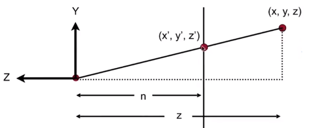
            And acording to the similar triangle we will get
            $$
            y’=\frac nz y，x’=\frac nz x
            $$
            So in homogeneous coordinatse
            $$
            \left(\begin{matrix}x\\y\\z\\1\end{matrix}\right)\rightarrow
            \left(\begin{matrix}\frac {nx}z\\\frac {ny}z\\unkown\\1\end{matrix}\right)==
            \left(\begin{matrix} nx\\ ny\\unkown\\z\end{matrix}\right)
            $$

         1. So the “squish” projection （ persp to ortho） does this
            $$
            M_{persp\rightarrow ortho}^{(4\times 4)}\left(\begin{matrix}x\\y\\z\\1\end{matrix}\right)
            =\left(\begin{matrix} nx\\ ny\\unkown\\z\end{matrix}\right)
            $$
            Already good enought to figure out part of $M_{persp \rightarrow ortho}$, and（By using matrices multyple）
            $$
            M_{persp \rightarrow ortho}=
            \left(\begin{matrix}
            n & 0 & 0 & 0
            \\
            0 & n & 0 & 0
            \\
            ? & ? & ? & ?
            \\
            0 & 0 & 1 & 0
            \end{matrix}\right)
            $$

         2. Observation: the third row is responsible for $z’$

            0. Any point on the near plane will not change
               $$
               M_{persp\rightarrow ortho}^{(4\times 4)}\left(\begin{matrix}x\\y\\z\\1\end{matrix}\right)
               =\left(\begin{matrix} nx\\ ny\\unkown\\z\end{matrix}\right)
               by\space replace \space z \space with \space n\space
               \left(\begin{matrix}x\\y\\z\\1\end{matrix}\right)\rightarrow
               \left(\begin{matrix}x\\y\\n\\1\end{matrix}\right)==
               \left(\begin{matrix} nx\\ ny\\n^2\\n\end{matrix}\right)
               $$
               So the third row must be of the form $（0\space 0\space A\space B）$ and
               $$
               （0\space 0\space A\space B）
               \left(\begin{matrix}x\\y\\z\\1\end{matrix}\right)=n^2​
               $$
               $n^2$ has nothing to do with $x$ and $y$ . Then we will get the equation $An+B=n^2$

               Any point’s $z$ on the far plane will not change: We will know that
               $$
               \left(\begin{matrix}0\\0\\f\\1\end{matrix}\right)\rightarrow\left(\begin{matrix}0\\0\\f\\1\end{matrix}\right)==\left(\begin{matrix}0\\0\\f^2\\f\end{matrix}\right)
               $$

               Then we will get the equation $Af+B=f^2$ .

            1. We will get a linear equations, by Cramer method ,we will solve this equations, and the answer are $A=n+f\space ,\space B=-nf$

            2. Finally, every coefficient we will know the matrix $M_{persp\rightarrow ortho}$

      2. What’s near plane’s $l,r,b,t$ then

         0. If explicitily specified, good

         1. Sometimes perople prefer: vertical field-of-view （fov$Y$）and aspect ratio（Assume symmetry）

         2. How to convert from fov$Y$ and aspect $l,r,b,t$？— Trivial

            
            $$
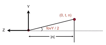
            tan\frac {fovY}2=\frac t{|n|},aspect=\frac rt
            $$

2. Rasterization

What’s after MVP?

Model transformation to place objects

View transformation to place camera

Projection transformation by Orthograpihc projection（cuboid to “canonical” cube $[-1,1]^3$ ）and Perspective projection （ frustum to “ canonical “ cube）

0. we should put Canonical Cube to Screen

   0. What is a screen?

      0. An array of pixels

      1. Size of the array: resolution

      2. A typical kind of raster display

   1. Raster == Screen in German

      Rasterize == drawing onto the screen

   2. Pixel（FYI, short for “picture element”）

      0. For now: A pixel is a little square with uniform color

      1. Color is a mixture of （red, green, blue）

   3. Defining the screen: Slightly different from the text “Tiger book”

      0. Pixels’ indices are in the form of $（x,y）$ where both $x$ and $y$ are integers

      1. Pixels’ indices are from $（0,0）$ to $（width-1,height-1）$

      2. But for every pixel （x,y）, the center of them are at $（x+0.5,y+0.5）$

      3. The screen covers range $（0,0）$ to $（width,height）$

      4. Irrelevant to $Z$

      5. Transform in $xy$ plane: $[-1,1]^2$ to $[0,width]\times [0,height]$, by using viewport transform
         $$
         M_{viewport}=
         \left(\begin{matrix}
         \frac {width}2 & 0 & 0 &\frac {width}2
         \\
         0 & \frac {height}2 & 0 & \frac{height}2
         \\
         0 & 0 & 1 & 0
         \\
         0 & 0 & 0 & 1
         \end{matrix}\right)
         $$

Rasterizing Triangles into Pixels

0. Some Drawing Machine and Different Raster Displays

   0. CNC sharpie Drawing Machine

   1. Oscilloscope（示波器）

      0. The principle: Cathode Ray Tube（阴极射线管）
      1. Televison: Raster Scan to get the image
      2. And it have some treat: Raster Scan Pattern of Interlaced Display（隔行扫描）

   2. Frame Buffer: Memory for a Raster Display

   3. Flat Panel Displays

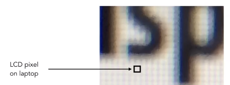
      0. LCD（Liquid Crystal Display） Pixel

         Principle :

         0. block or transmit light by twisting polarization
         1. Illumination from backlight
         2. Intermediate intensity levels by partial twist

      1. LED（Light emitting diode）

      2. Electrophoretic（Electronic ink）Display

1. Rasterization: Drawing to Raster Displays

   Triangles - Fundamental Shape Primitives.

   0. Why Triangles?

      0. Most basic polygon —— Break up other polygons
      1. Unique properties —— Guaranteed to be plannar, well-defined interior and well-defined method for interpolation values at vertices over triangle （Barycentric interpolation）

   1. What Pixel Values Approximate a Triangle?

      Input position of triangle vertices projected on screen, how to outpoot?

      0. Sampling a Function: Evaluating a function at a point is sampling. We can discretize a function by sampling

          for （int i=0;i<xmax;x++） 
              output[x]= f（x）;

   2. Samplng is a core idea in graphics: We sample time（1D）, area（2D）, direction（2D）,volume（3D）and etc.

      2. Sample if Each Pixel Center is Inside Triangle - Define binary function

         bool inside（tri t, Point p）;
         //struct Point {
         //    Elementtype x, y;
         //};
         //x,y not necessarily integers
         //if Point p（x,y） in the t,return true
         //else return false

      3. Rasterization = Sampling A 2D Indicator Function（The main code as follow）

         for （int x = 0; x < xmax; ++x）
             for（int y = 0; y< ymax; ++y）
                 image[x][y]=inside（tri,
                                    x + 0.5,
                                    y + 0.5）;

      4. Another way to judge a point whether in the triangle: Use Cross Product:

         Suppose $3$ points $A,B,C$, the point $Q$ we want to judge

         We can get $3$ vectors $\vec {AQ},\vec {BQ},\vec {CQ}$

         If all the $\vec {AB}\times \vec {AQ},\vec {CA} \times \vec {CQ},\vec {BC}\times \vec {BQ}$ are positive or negative, the point in the triangle.

         Else not in the triangle.

      5. Edge Cases : We omit it. But if you want to make some special check, you should treatment it special.

      6. We can take some method to decrease some calculate like bounding box and etc.

2. Rasterization on Real Displays

   0. Example: Real LCD Screen Pixels （Closeup）（The second called Bayer Pattern）

   1. Real_LCD

      

      We can see that the green part more than red and blue, because of the more sensitive to green for our eyes.

   2. Other Display Methods

      

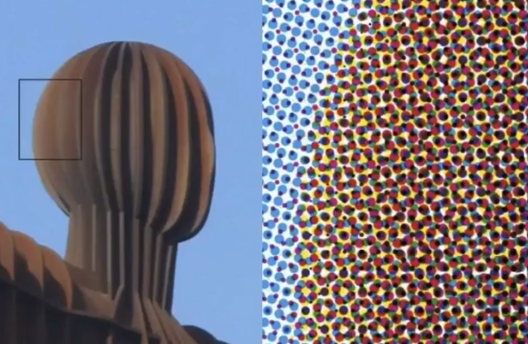
3. Assume Display Pixels Emit Square of Light

   

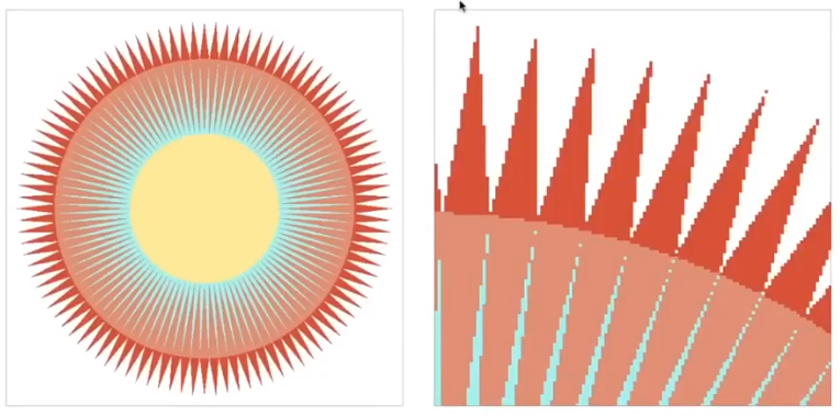
Antialiasing

0. Sampling theory

   Sampling is Ubiquitous in CG

   0. Rasterization = Sample 2D Positions

   1. Photograph = Sample Image Sensor Plane

   2. Video = Sample Time

   Sampling Artifacts（Erros / Mistakes / Inaccuracies ） in CG

   0. Jaggies （Stair case Pattern）

      

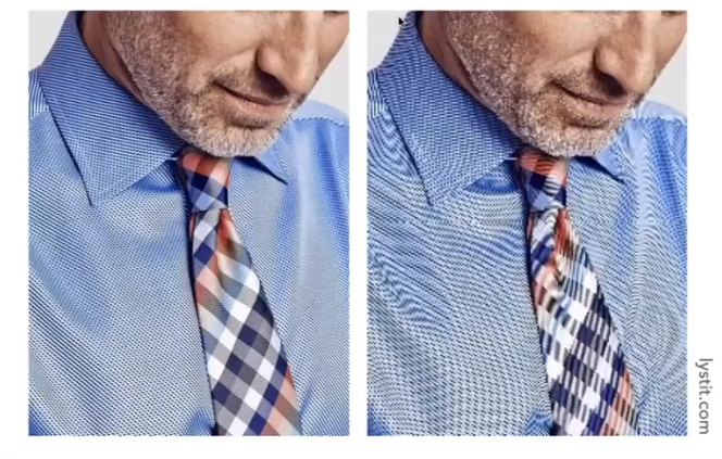
   1. Moire Patterns in Imaging

      

   2. Wagon Wheel Illusion （False Motion）

   3. And Many More

      Behind the Aliasing Artifacts:

   Signals are changing too fast （ high frequency ）but sampled too slowly.

1. Antialiasing Idea: Blurring （Pre - Filtering） Before Sampling

   0. Rasterization: Point Sampling in Space
   

   This is Regular Samping, Note jaggies in rasterized triangle where pixel value are pure red or white

   1. Pre-Filter

      

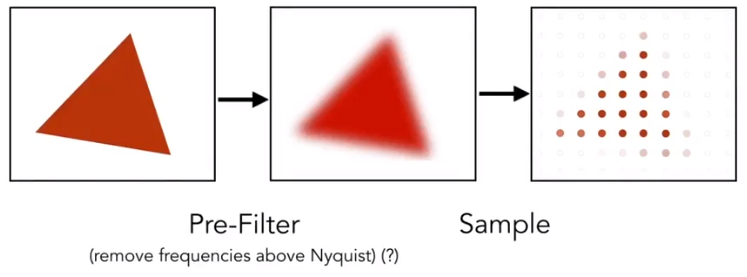
      This is *Antialiased Sampling *. Note antialiased edges in rasterized triangle wher pixel values take intermediate values.

   2. But we can’t sample then filter will lead to “Blurred Aliasing“

      

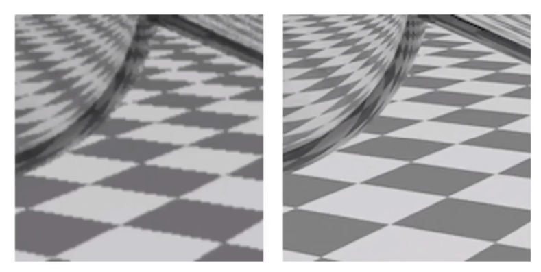
      The first is sample then filter, the second is right.

      0. Why undersampling introduces aliasing and why pre-filtering then sampling can do antialiasing?

         0. Frequency Domain

            0. $sin\omega x$ and $cos\omega x$： well-know periodic functions, the periodic, $f$ is frequency.
               $$
               f=\frac \omega {2\pi}
               $$

            1. Fourier Series Expansion: For every periodic functions, it can be written as a linear combination of sine and cosine.

            2. Fourier Transform: spatial domain function $f（x）$ can be transform by Fourier transform $F（\omega）=\int_{-\infty}^{\infty}f（x）e^{-2\pi i\omega x}dx$ to frequency domain $F（\omega）$, and according to Euler Formular $e^{ix}=cosx+isinx$.

            3. Inverse transform: From $F（\omega）$ by $f（x）=\int_{-\infty}^{\infty}F（\omega）e^{2\pi i \omega x}d\omega$ to $f（x）$

         1. Sampling emulation: Higher Frequencies Need Faster Sampling

            Undersampling Creates Frequency Aliases: High-frequency signal is insufficiently sampled: samples erroneously appear to be from a low-frequency signal.

            Two frequencies that are indistinguishable at a given sampling $f$ are called “aliases”（混叠）

         2. Filtering = Getting rid of certain frequency contents

            0. Example: Visualizing Image Frequency Content

               

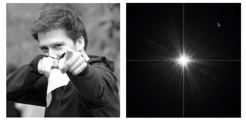
               We can know that the lowest frequency information are gathered in the center of the image, and the brighter the color, the more information there is. So this image has many low frequency information. The frequency around are the detail of the image.（Many natural picture like this.）

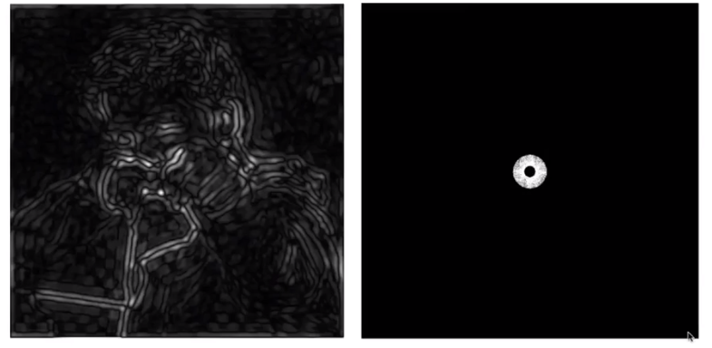
            1. Filter out Low Frequencies Only（Edges）

               

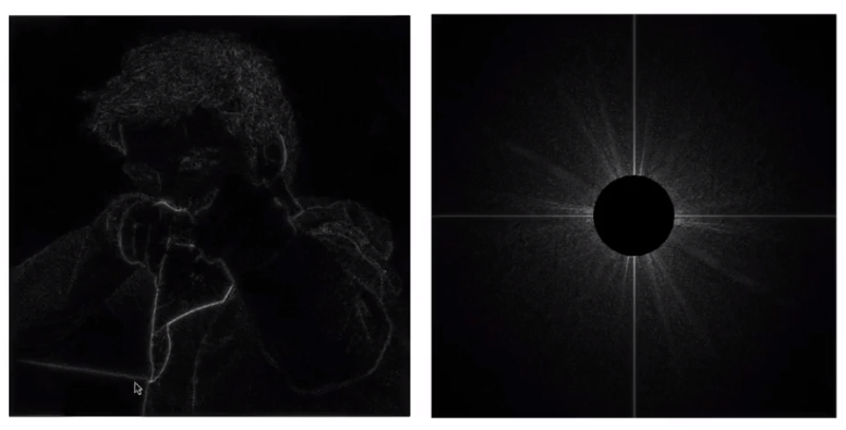
            2. Filter Out High Frequencies（Blur）

               

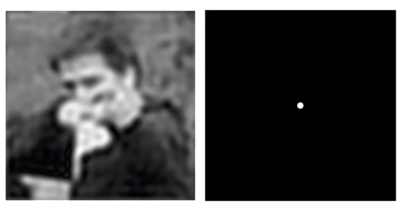
            3. Filter Out Low and High Frequencies

               

         3. Filtering = Convolution = Average

            In a word, convolution can see it as the “average“ in frequency domain and the average can see it as the average in spatial domain

            0. Convolution

               Given a signal sequence $S=[1,3,5,3,7,1,3,8,6,4$ , and a filter $F=[\frac 14,\frac 12,\frac 14]$, the result of the convolution about signal and filter can get a sequence $R$. The $i-th$ element in the result sequence can be caculate by
               $$
               R[i]=S[i-1]\times F[1]+S[i]\times F[2]+S[i+1]\times F[3]
               $$
               The procesion of it is convolution.

            1. Convolution Theorem: Convolution in the spatial domain is equal to mulitiplication in the frequency domain , and vice versa

               0. Filter by convolution in the spatial domain

               1. Thansform to frequency domain（Fourier tansform）, multiply by Fourier transform of convolution kernel and Transform back to spatial domain（Inverse Fourier）

               2. Example:

                  

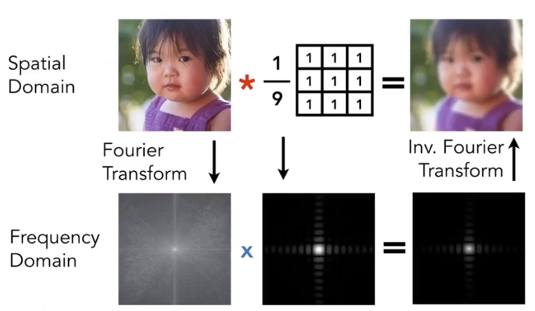
               3. Box Filter = “Low Pass Filter”
                  $$
                  \frac 19 \left[ \begin{matrix}1&1&1\\1&1&1\\1&1&1\end{matrix}\right]
                  $$

               4. Wider Filter Kernel = Lower Frequencies

         4. Sampling = Repeating Frequency Contents

         5. Aliasing = Mixed Frequency Contents

            

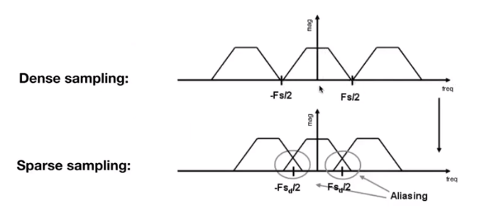
   3. Reduce Aliasing Error

      0. Increase sampling rate

         0. Essentially increasing the distance Essentially increasing the distance between replicas in the Fourier domain

         1. Higher resolution displays, sensors, framebuffers…

         2. But: costly & may need very high resolution

      1. Antialiasing: making Fourier contents “narrower” brfore repeating

         0. Antialiasing = Limiting then repeating

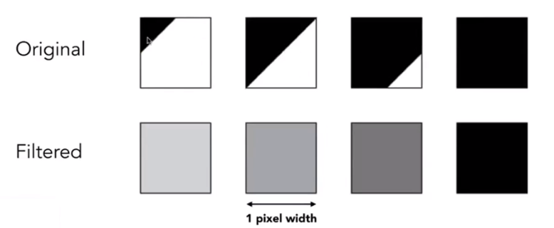
         1. Antialiasing By Averaging Values in Pixel Area

            Solution: Convolve $f（x,y）$ by a $1$-pixel box-blur, Then sample at every pixel’s center

         2. Example: Antialiasing by Computing Average Pixel Value

            In rasterizing one triangle, the average value inside a pixel area of $f（x,y）= $inside（triangle,point） is equal to the area of the pixel covered by the triangle.

            

      2. Antialiasing By Supersampling （MSAA）

         0. Supersampling

            Approximate the effect of the 1-pixel box filter by sampling multiple locations within a pixel and averaging their values

         1. Example

            0. Beginning

               

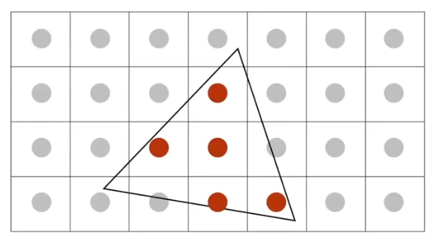
            1. First Step: Take $N\times N$ samples in each pixel

               

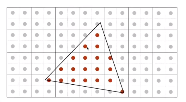
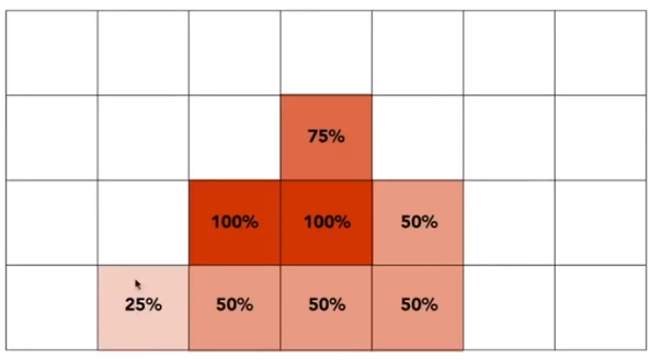
            2. Second Step: Average the $N\times N$ samples “inside” each pixel

               

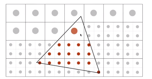
            3. then

               

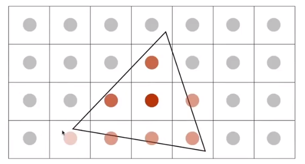
            4. Result: This is the corresponding signal emitted by the display, but MSAA doesn’t increase the dpi

               

         2. No free lunch!

            What’s the cost of MSAA? More calculate and more buffer.

         3. Milestones

            0. FXAA（Fast Approximate AA）（快速近似反走样）

               No relationship with add more sample, it is the post-processing of the image. It changes the edge with jaggies to non-jaggy edge . It is quickly.

            1. TAA（Temporal AA） /tem’pərəl/

               To get the post frame information and change some of this frame’s value.

         4. Super resolution（超分辨率） / super sampling

            0. From low resolution to high resolution
            1. Essentially still “not enough samples” problem
            2. DLSS（Deep Learning Super Sampling）

Visibility / occlusion - Z-Buffer

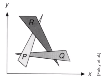
0. Painter’s Algorithm - Inspired by how painters paint.

   Paint from back to front, overwrite in the framebuffer. It requires sorting in depth （$O(nlogn)$） for n triangles. But it can have unresolvable depth order, for example

   

1. Z-Buffer- This is the algorithm that eventually won,

   0. Idea:

      0. Store current min.z-value for each sample（pixel）
      1. Needs an additional buffer for depth values
         0. Frame buffer stores color values
         1. Depth buffer（z-buffer）stores depth

   1. IMPORTANT:

      For simplicity we suppose, z is always positive（smaller z$\rightarrow$closer, larger z$\rightarrow$further）

   2. Example

      

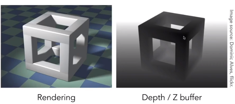
   3. Pseudocode

      Initialize depth buffer to $\infty$, and during rasterization

      for(each triangle T)
          for(each sample (x, y, z) in T){
              if(z < zbuffer[x,y]){       // closest sample so far
                  framebuffer[x,y] = rgb; // update color
                  zbuffer[x,y] = z;       // update depth
              } 
              else ;// do nothing, this sample is occluded
          }

   4. Complexity

      0. $O(n)$ for $n$ triangles (assuming constant coverage).
      1. “Sort” $n$ triangles in linear times, because we just find the minimum value,

   5. Triangles in different orders, it will have same appearance.

   6. Most important visibility algorithm - Implemented in hardware for all GPUs

3. Shading

The definition of the shading in Merriam-Webster Dictionary is that the darkening or coloring of an illustration or diagram with parallel lines or a block of color.

In this course, the process of applying a meterial to an object is shading

A Simple Shading Model - Blinn-Phong Reflectance Model

0. Perceptual Observation

1. Shading in Local:

   Compute light reflected toward camera at a specific shading point

   0. Inputs:

      
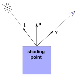
      0. Viewer direction $\vec v$
      1. Surface normal $\vec n$
      2. Light directions $\vec L_i$
      3. Surface parameters such as color, shininess and etc

   1. No shadows will be generated!（ shading $\neq$ shadow ）

   2. Diffuse Reflection（Blinn-Phong）

      0. Light is scattered uniformly in all directions - Surface color is the same for all viewing directions

      1. Lambert’s cosine law

         

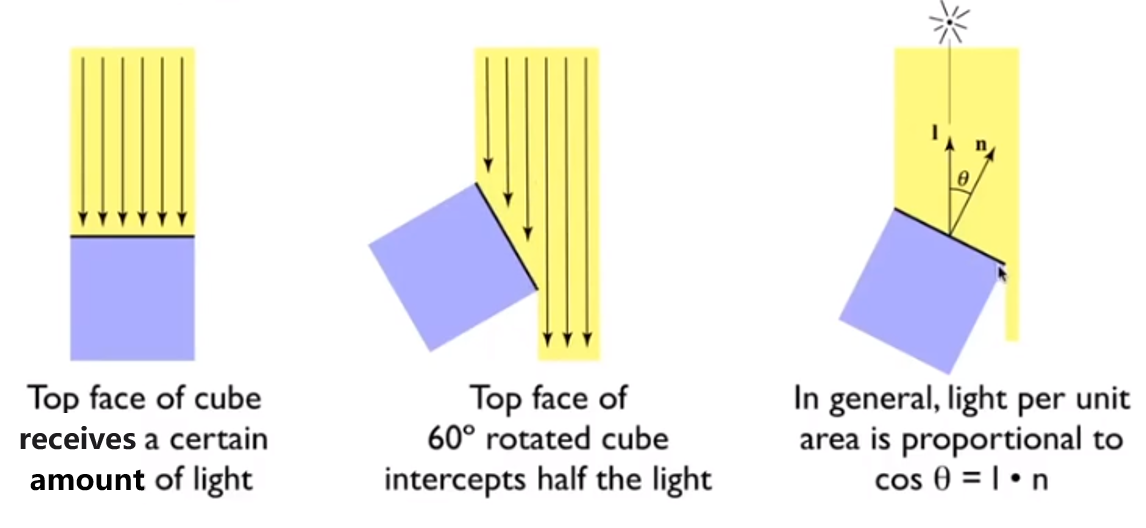
      2. Light Falloff

         Assume there is a loop with $r=1$, the light source in the center, then the intensity here is $I$.

         If when suppose the distance of the center and a point is $r$, then the intensity here is
         $$
         \frac I{r^2}
         $$

      3. Lambertian（Diffuse）Shading

         Shading independent of view direction, we will have
         $$
         L_d=k_d\frac I{r^2} max(0,\vec n \cdot \vec l)
         $$
         where

         ​ $L_d$ is diffusely reflected light

         ​ $k_d$ is diffuse coefficient（color）

         ​ $max(0,\vec n \cdot \vec l)$ is energy received by the shading point, 0 can avoid the negative value

   3. Specular Term（Blinn-Phong）

      0. Intensity depends on view direction - Bright near mirror reflection direction

      1. $V$ close to mirror direction == half vector near normal

         

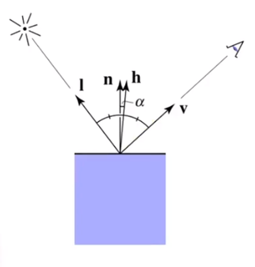
         Measure “near” by dot product of unit vectors, and we get this vector
         $$
         \vec h = bisector(\vec v, \vec l)=\frac{\vec v + \vec l}{||\vec v + \vec l||}\\
         L_s=k_s\frac I{r^2}max(0,\vec n \cdot\vec h)^p
         $$
         Where

         ​ $L_s$ is secularly reflected light

         ​ $k_s$ is specular coefficient

         Be care for that $max(0,\vec n \cdot\vec h)^p$ have pow $p$, because the cosine function have a property that increasing p narrows the refection lobe.

   4. Ambient Term

      Shading that does not depend on anything

      0. Add constant color to account for disregarded illumination and fill in black shadows

      1. This is approximate / fake
         $$
         L_a=k_aI_a
         $$
         Where

         ​ $L_a$ is reflected ambient light

         ​ $k_a$ is ambient coefficient

   5. Blinn-Phong Reflection Model

      
      $$
      L=L_a+L_d+L_s
      =k_aI_a+L_d=k_d\frac I{r^2} max(0,\vec n \cdot \vec l)+k_s\frac I{r^2}max(0,\vec n \cdot\vec h)^p
      $$

Shading Frequencies

0. Shade each triangle（Flat shading）

   0. Triangle face is flat - one normal vector
   1. Not good for smooth surfaces

1. Shade each vertex（Gouraud shading）

   0. Interpolate colors from vertices across triangle
   1. Each vertex has a normal vector

2. Shade each pixel（Phong shading）

   0. Interpolate normal vectors across each triangle
   1. Compute full shading model at each pixel
   2. Not the Blinn-Phong Reflectance Model

3. Defining Per-Vertex Normal Vectors

   0. Best to get vertex normals from the underlying geometry.

   1. Otherwise have to infer vertex normals from triangle faces, such like
      $$
      N_v=\frac {\sum _iN_i}{||\sum_iN_i||}
      $$

      

   2. Barycentric interpolation of vertex normals

      

   3. Don’t forget to normalize the interpolated directions

Barycentric Coordinates - Interpolation Across Triangles

0. Some Problems

   0. Why do we want to inerpolate

      Specify values at vertices and Obtain smoothly varying values across triangles

   1. Wahat do we want to interpolate

      Texture coordinates, colors, normal vectors. …

   2. How do we interpolation

1. Barycentric Coordinates

   A coordinate system for triangles $(\alpha, \beta,\gamma)$. For any triangle $ABC$ , assume there is a point $p(x,y)$, then we will get this equation（Inside the triangle if all three condinates are non-negative）
   $$
   (x,y)=\alpha A+\beta B+ \gamma C\\
   \alpha +\beta +\gamma = 1
   $$
   And in the formula, we can get follows accoding to the picture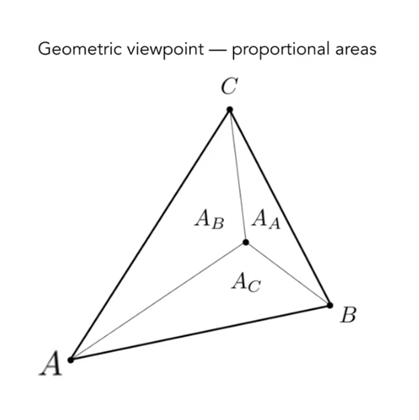

   

   Then
   $$
   \alpha =\frac {A_A}{A_A+A_B+A_C}
   \\
   \beta =\frac {A_B}{A_A+A_B+A_C}
   \\
   \gamma=\frac {A_C}{A_A+A_B+A_C}
   $$

2. Barycentric Coordinates：$\alpha =\beta =\gamma = \frac 13$

3. Barycentric Coordinates： Fomulas
   $$
   \alpha=\frac{-(x-x_B)(y_C-y_B)+(y-y_B)(x_C-x_B)}{-(x_A-x_B)(y_C-y_B)+(y_A-y_B)(x_C-x_B)}
   \\
   \beta=\frac{-(x-x_C)(y_A-y_C)+(y-y_C)(x_A-x_C)}{-(x_B-x_C)(y_A-y_C)+(y_B-y_C)(x_A-x_C)}
   \\
   \gamma=1-\alpha -\beta
   $$

4. Using interpolate values at vertices
   $$
   V=\alpha V_A+\beta V_B+\gamma V_C
   $$
   where $V_A,V_B,V_C$ can be positions, texture coordinates, color, normal, depth, material attributes…

   But barycentric coordinates are not invariant under projection!

Graphics （Real-time Rendering）Pipeline

A picture can conclude it briefly。

Shader Programs

0. Program vertex and fragment processing stages

1. Describe operation on a single vertex（or fragment）

2. Example GLSL fragment shader program

   uniform sampler2D myTexture;
   uniform vec3 lightDir;
   varying vec2 uv;
   varying vec3 norm;
   
   void diffuseShader()
   {
       vec3 kd;
       kd = texture2d(myTexture, uv);
       kd *= clamp(dot(-lightDir, norm), 0.0, 1.0);
       gl_FragColor = vec4(kd, 1.0);
   }

3. Some tips

   0. Shader function executes once per fragment
   1. Output color of surface at the current fragements screen sample position
   2. This shader perform a texture lookup to abtain the surface’s material color at this point, then performs a diffuse lighting calculation

Texture Mapping

0. Surfaces are 2D

   Surface lives in 3D world space, but every 3D surface point also has a place where it goes in the 2D image（Texture）

1. Visualization of Texture Coordinates

   Each triangle vertex is assigned a texture coordinate $（u,v）,u,v\in [0,1]$

2. Apllying Textures

   0. Simple Texture Mapping - Diffuse Color

      for each raterized screen sample (x,y):   //Usually a pixel's center
          (u,v) = evaluate texture coordinate at (x,y)  //using barycentric coordinates
           texcolor = texture.sample(u,v);
           set sample's color to texcolor;     //Usually the diffuse albedo Kd

   1. Texture Magnification

      0. Easy Case

         Generally don’t want this — insufficient texture resolution, a pixel on a texture — a texel（纹理元素), and look at the picture

         

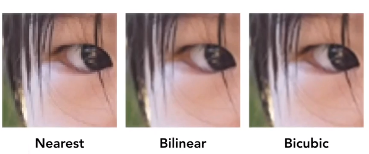
      1. Bilinear Interpolation

         If we want to sample textture value $f(x,y)$ at a point. and there are some points ${P_{blacki}}$ indicate texture sample locations.

         We can take 4 nearest sample locations, with texture valus as labeled ${u_{0i}}$, and fractional offsets $(s,t)$ as $(distance(u_{00},x),distance(u_{00},y))$

         Linear interpolation（1D）
         $$
         lerp(x,v_0,v_1)=v_0+x(v_1-v_0)
         $$
         Two helper lerps
         $$
         u_0=lerp(s,u_{00},u_{10})
         \\
         u_1=lerp(s,u_{01},u_{11})
         $$
         Find vertical lerp, to get result:
         $$
         f(x,y)=lep(t,u_0,u_1)
         $$
         Bilinear interpolation usually gives pretty good results at reasonable costs.

      2. Hard Case

         

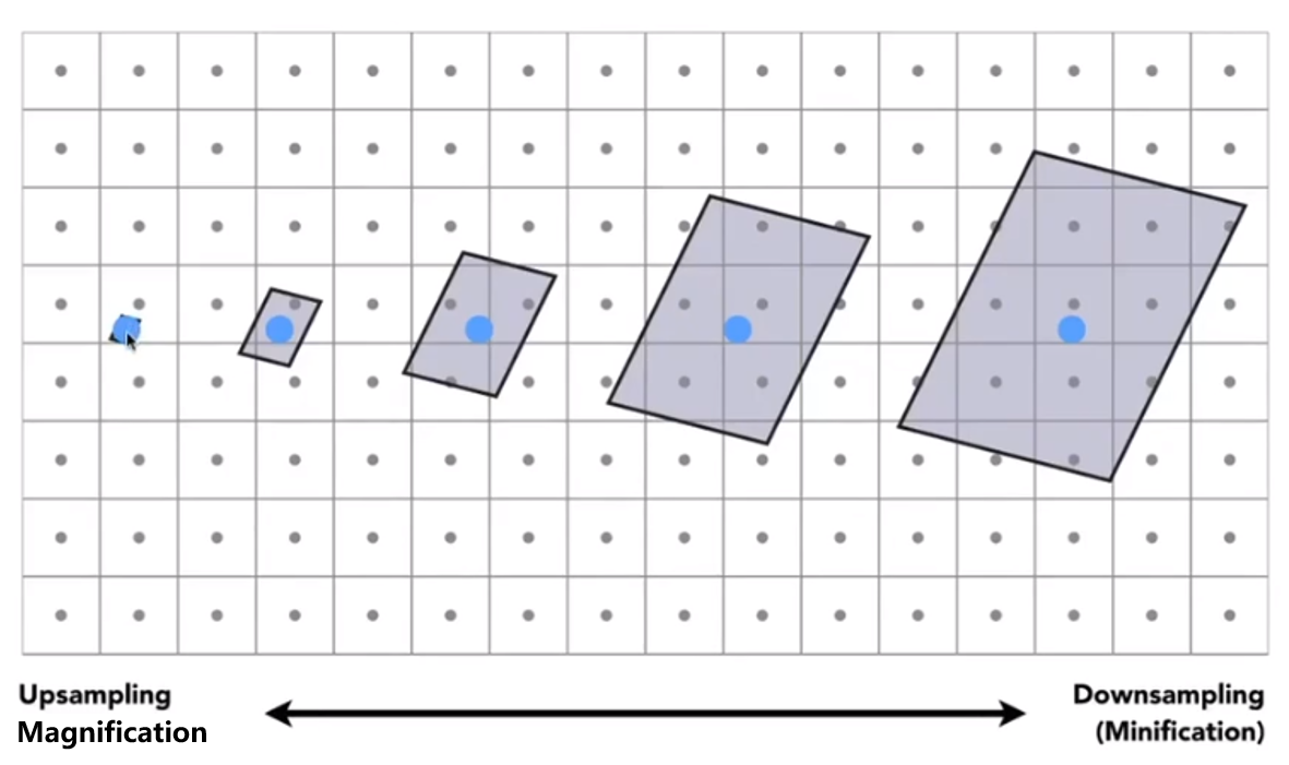
         0. Screen Pixel “Foortprint” in Texture

            

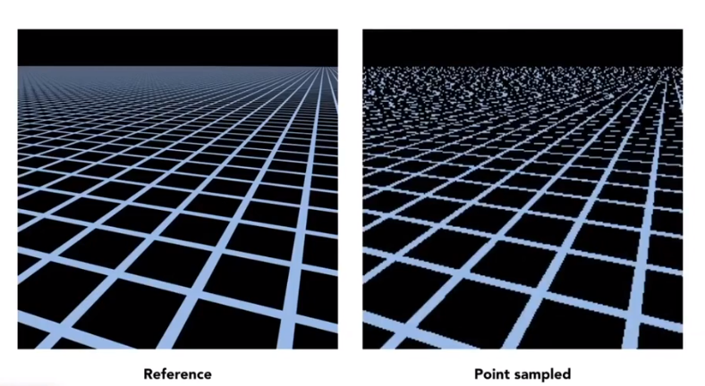
         1. Will supersampling Do Antialiasing?

            Yes! But costly

            0. When highly minified, many texels in pixel footprint
            1. Signal frequency too large in a pixel
            2. Need even higher sampling frequency

         2. So what if we don’t sample?

            Just need to get the average value within a range！

      3. Mipmap

         0. Mipmap - Allowing （fast, approx., square）range queries

            “Mip” comes from the Latin “Multum in parvo”, meaning a multitude in a small space, for example

            

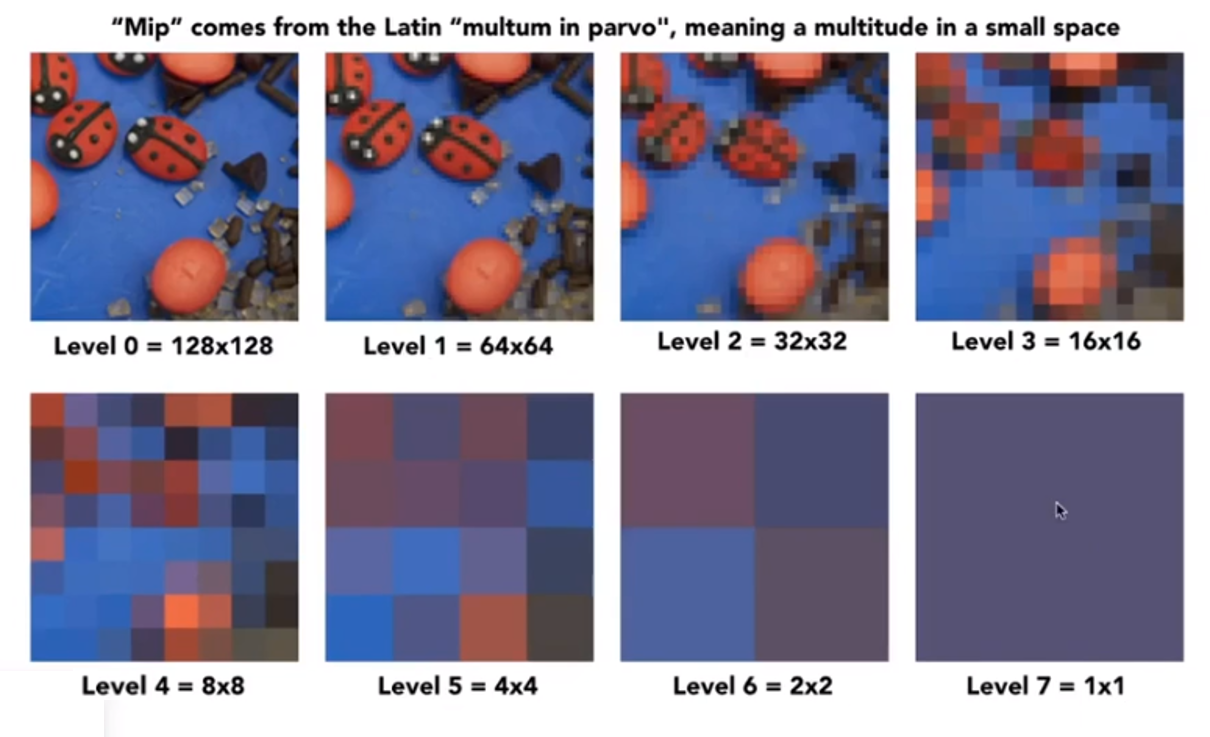
            and we will get “Mip hierarchy（level = D）”

            

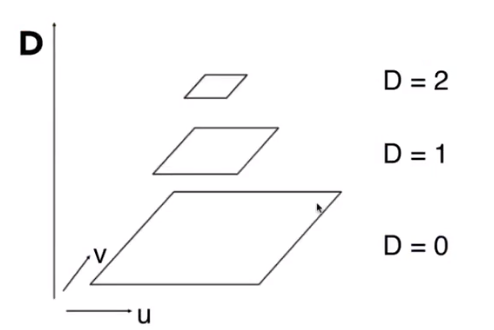
            The buffer we need is about 1.33 times than before.

         1. Computing Mipmap Level D

            

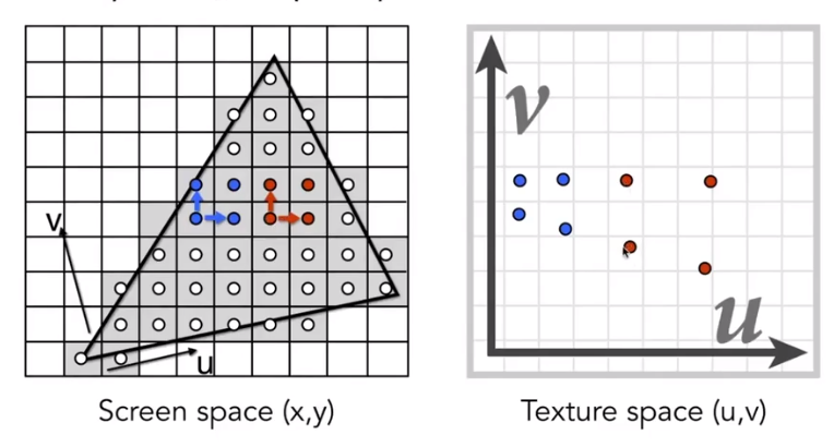
            then

            

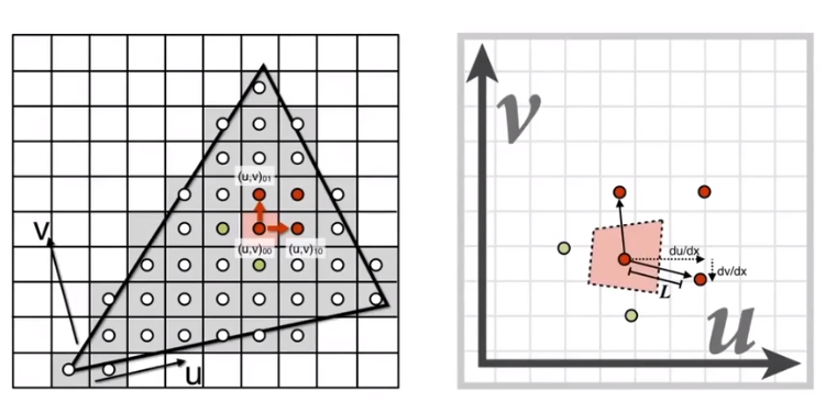
            We will get
            $$
            D=log_2L\\L=max\left(\sqrt{(\frac {du}{dx})^2+(\frac {dv}{dx})^2}, \sqrt{(\frac {du}{dy})^2+(\frac {dv}{dy})^2}\right)
            $$
            and then use square approximate the origin area

            

         2. Trilinear Interpolation = Bilinear result（in the same level）+Bilinear result（In the adjacent level）

         3. Mipmap Limitations - Overblur

            Anisotropic Filtering: Ripmaps and summed area tables

            0. Can look up axis-aligned rectangulare zones
            1. Diagonal footprintfs still a problem

            EWA filtering

            0. Use multiple lookups
            1. Weighted average
            2. Mipmap hierarchy still helps
            3. Can handle irregular footprints

Applications of textures

In modern GPUs, texture = memory + range query（Filtering）. And General method to bring data to fragment calculations.

So it have many usages

0. Environment lighting: Spherical Map then Cube Map

1. Store microgeometry: Fake the detailed gemoetry by bump / normal mapping

   0. Bump Mapping: Adding surface detail without adding more triangles

      Note that this is in local coordinate!

      0. Perturb surface normal per pixel（For shading computations only）

         Original surface normal $n(p)=(0,1)$

         Derivative at $p$ is $dp=c\times [ h(p+1)-h(p)]$

         Pertubed normal is then $n(p)=(-dp,1).normalized()$

      1. In 3D

         Original surface normal $n(p)=(0,0,1)$

         Derivative at $p$ are $\frac {dp}{du}=c_1\times [ h(u+1)-h(u)]$; $\frac {dp}{dv}=c_1\times [ h(v+1)-h(v)]$

         Pertubed normal is then $n(p)=(-\frac {dp}{du},-\frac {dp}{dv},1).normalized()$

      2. “Height shift” per texel defined by a texture

      3. Modify normal vector

   1. Displacement mapping - a more advanced approach

      Uses the same texture as in bumping mapping

      Acturally move the vertices

2. Procedural textures

3. Solid modeling

   Example: 3D Procedural Nosie + Solid Modeling (Perlin Noise)

4. Volume rendering

5. Provide Precomputed Shading

6. And etc.

4. Geometry

Introduction

0. Examples of Geometry

1. Rresent Geometry

   0. Implicit: Based on lassifying points

      0. method:

         0. Algebraic surfaces,

         1. Level sets

            0. Closed-form equations are hard to describe complex shapes
            1. Alternative: store a grid of values approximating function
            2. Surface is found where interpolated values equal zero
            3. Provides much more explicit control over shape (like a texture)

         2. Distance functions

            Giving minimum distance （could be distance） from anywhere to object

         3. Constructive Solid Geometry

            Bool operate among some geometry.

         4. Fractals（分形）

         5. and etc

      1. Points satisfy some specified relationshp, example $x^2+y^2+z^2=1$ is a ball. More generally, $f(x,y,z)=0$

      2. Disadvantage is sampling can be hard

      3. Advantage is easy to judge a point inside/outside

   1. Explicit: All points are given directly or via parameter mapping

      0. method:

         0. point cloud: Easiest representation: list of points $(x,y,z)$, it can easily represent any kind of geometry. It usually useful for large datasets, often converted into polygon mesh and difficult to draw in undersampled regions.

         1. polygon mesh: Store vertices & polygons （often triangles or quads）. It is easier to do processing / simulation, adaptive sampling, more complicated data structures. Perhaps most common representation in graphic.

            The Wavefront Object File (.obj) Format, a commonly used in Graphics research. Just a text file that specifies vertices, normals, texture coordinates and their connectivities.

         2. subdivision, NURBS

         3. and etc

      1. Example: $f: \mathbb R^2 \rightarrow \mathbb R^3；(u,v)\mapsto (x,y,z) $

      2. Disadvantage is hard to judge a point inside/outside

      3. Advantage is sampling is easy

   2. Each choice best suited to a different task / type of geometry

   3. Best Representation Depends on the Task

2. Implicit Representations

   0. Pro
      0. compact description （ such like a function）
      1. certain queries easy （inside object, distance to surface）
      2. good for ray-to-surface intersection（more later）
      3. for simple shapes, exact description / no sampling error
      4. easy to handle changes in topology (e.g. fluid)
   1. Cons
      0. difficult to model complex shapes

curves

0. Bezier Curves： Defining Cubic Bezier Curve With Tangents

   

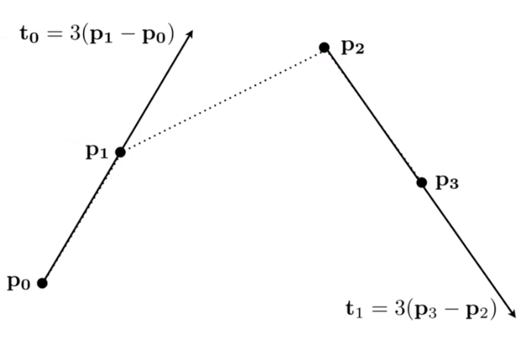
   We can easy know that the beginning and ending is $p_0$ and $p_3$.

1. Evaluating Bezier Curves（de Casteljau Algorithm）

   Consider three points（quadratic Bezier）, insert a point using linear interpolation and recursively.

   

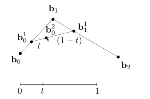
   and then link the point smoothly and you will get

   

   It can be use in more points.

2. Evaluating Bezier Curves Alegbraic Formula

   0. de Casteljau algorithm gives a pyramid of coefficients

      

      then we will get some formulas
      $$
      b_0^1(t)=(1-t)b_0+tb_1\\
      b_1^1(t)=(1-t)b_1+tb_2\\
      b_0^2(t)=(1-t)b_0^1+tn_1^1
      =(1-t)^2b_0+2t(1-t)b_1+t^2b_2
      $$
      It is Bernstei form of a Bezier cureve of order n:
      $$
      b^n(t)=b_0^n(t)=\displaystyle\sum_{j=0}^nb_jB_j^n(t)
      $$
      where

      ​ $b^n(t)$ is bezier curve order $n$（vector polynomial of degree $n$）

      ​ $b_j$ is Bezier control points（vector in $\mathbb R^n$）

      ​ $B_j^n(t)$ is Bernsterin polynomial（scalar polynomial of degree $n$）

      And Bernstein polynomials
      $$
      B_i^n(t)= {n\choose i}t^i(1-t)^{n-i}
      $$
      So the Bernstein form of a Bezier curve of order $n$
      $$
      b^n(t)=\displaystyle\sum_{j=0}^nb_jB_j^n(t)
      $$
      For example, in $\mathbb R^3$ and $n=3$, $b_0=(0,2,3), b_1=(2,3,5), b_2=(6,7,9),b_3=(3,4,5)$

      These points define a Bezier curve in 3D that is a cubic polynomial in $t$
      $$
      b^n(t)=b_0(1-t)^3+b_13t(1-t)^2+b_23t^2(1-t)+b_3t^3
      $$

   1. Bernstein Polynomials

      

   2. Properties of Bezier Curves

      0. Interpolates endpoints

         $b(0)=b_0,b(1)=b_{end}$

      1. Tangent to end segments

         $b’(0)=k(b_1-b_0);b’(1)=k(b_{end}-b_{end-1})$

      2. Affine transformation property

         Transform curve by transforming contro points

      3. Convex hull property

         Curve is within convex hull of control points

         

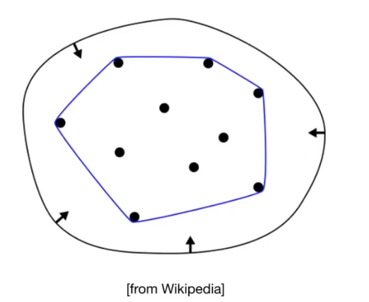
3. Piecewise Bezier Curves

   If $n$ is big, it will very hard to control. Instead, chain many low-order Bezier curve.

   Piecewise cubic Bezier the most common technique

   0. Continuity

      

      $C^0$ continuity: $a_n=b_0$

      $C^1$ continuity:$a_n=b_0=\frac 12(a_{n-1}+b_1)$

4. Spline

   A continuous curve constructed so as to pass through a given set of points and have a certain number of continuous derivatives. In short, a curve under control

5. B-splines

   Short for basis splines

   Require more information than Bezier curves

   Satisfy all important properties that Bezier curves have (i.e. superset)

   It’s hard to explain, if you want to know more, you can see my article “清华MOOC图形学基础：几何造型”

surfaces

0. Bezier Surfaces

   0. Bicubic Bezier Surface Patch : Use Bezier Curve in two direction.

   1. Evaluating Bezier Surfaces:

      For bicubic Bezier surface patch

      ​ Input ：$4\times 4$ control points

      ​ Output：2D surface parameterized by $(u,v)$ in $[0,1]^2$

      ​ Goal: Evaluate surface position corresponding to $(u,v)$

      ​ $(u,v)$-separable application of de Casteljau algorithm

      0. Use de Casteljau to evaluate point u on each of the 4 Bezier curves in $u$. This gives 4 control points for the “moving” Bezier curve.
      1. Use 1D de Casteljau to evaluate point $v$ on the “moving” curve

1. Mesh Operations：Geometry Processing

   0. Mesh subdivision - Increase resolution

      

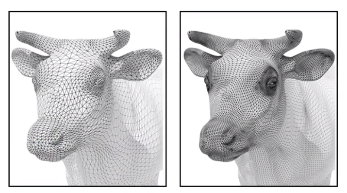
      0. Loop Subdivision（Loop is a person）

         Common subdivision rule for triangle meshs.

         First, create more triangles（vertices）, second, tune their positions

         Split each triangle into four, then assign new vertex positions according to weights（New / old vertices updated differently）

      1. Loop subdivision - Update

         For new vertices: we name 2 equilateral triangles’ vertices as $A,B,C$ and $A,B,D$. Then, we find a new vertex in $AB$, and the position should follow $\frac 38\times(A+B)+\frac 18\times (C+D)$

         For old vertices: the point in the center of the degree 6 vertices will update to the point which follow the rule ($u$ is the old vertices )$(1-n\times u)\times original_position+u\times neighbor_position_sum$

      2. Catmull-Clark Subdivision（General Mesh）

         

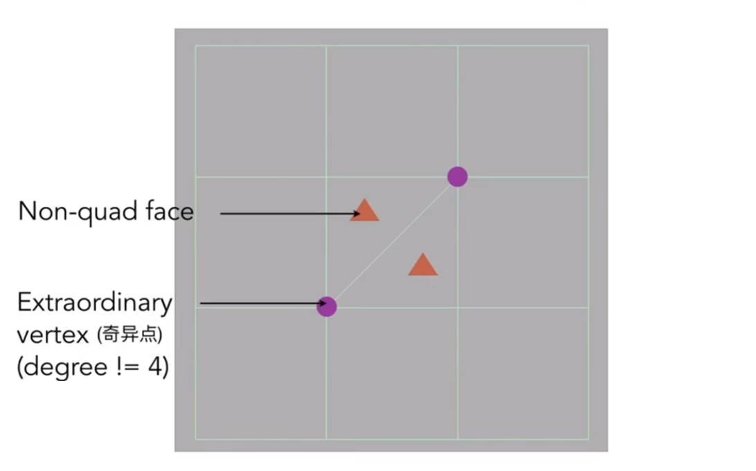
         Each subdivision step: Add vertex in each face. Add midpoint on each edge and connect all new vertices.

         After one subdivision: There have 4 extraordinary vertices, and their degrees are 3（new） or 5（old）and there have no non-quad faces.

         FYI： Catmull-Clark Vertex Update Rules（Quad Mesh）

         Face point：
         $$
         f=\frac {v_1+v_2+v_3+v_4}4
         $$
         Edge point:
         $$
         e=\frac {v_1+v_2+f_1+f_2}4
         $$
         Vertex point
         $$
         e=\frac {f_1+f_2+f_3+f_4+2(m_1+m_2+m_3+m_4)+4p}{16}
         $$
         The convergence of Catmull-Clark Subdivition can overall shape and creases.

   1. Mesh simplification - Decrease resolution; try to preserve shape / appearance

      

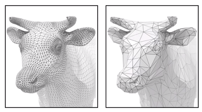
      0. Gold：Reduce number of mesh elements while maintaing the overall shape
      1. Method：Collapsing An Edge - Suppose we simplify a mesh using edge collapsing
         0. Quadric Error Metrices: New vertex ahould minimize its sum of square distance（L2 distance） to previously related triangle planes.
         1. How ie cost to collapse an edge: computing edge midpoint, measure quadric error
         2. Simplification via Quadric Error：Iteratively collapse edges
            0. approximate distance to surface as sum of distances to planes containing tricangles.
            1. iteratively collapse edge with smallest score
            2. use priority queue and some greedy algorithm

   2. Mesh regularization - modify sample distribution to improve quality

      

2. Shadow mapping

   0. An Image-space Algorithm

      0. no knowledge of scene’s gfeometry during shadow computation

      1. must deal with aliasing artifacts

   1. Key idea

      The points Not in shadow must be seen both by the light and by the camera

   2. Step 1：Render from Light：Depth image from light source

   3. Step 2A：Render from eye：standard image （with depth） from eye

   4. Step 2B：Project to light：Project visible points in eye vie back to light source

      Note: Reprojected depths from light and eye may not the same, so in some cases, we should BLOCKED it

   5. The example you can see the BV1X7411F744?t=1323&p=12 beginning with 60’10’’

   6. Problem with shadow maps

      0. Hard shadows（points lights only）

         Be care for that if the light source have volume, it can be generate soft shadows by other methods, but if it is a point ,it can only generate hard shadows

      1. Quality depends on shadow map resolution（general problm with image-based techniques）

      2. Involves equality comparison of floating point depth values means issues of scale, bias, tolerance

5. Ray Tracing

Why Ray Tracing?

0. Becase rasterization couldn’t handle global effects well, like（soft） shadows and especially when the light bounces more than once

1. Rasterization is fast, but quality is relatively low

2. Ray tracing is accurate, but is very slow

   Rasterization：real-time, but ray tracing is offline, and it will use about 10K CPU core hours to render one frame in production.

Light Rays - Three ideas about light rays

0. Light travels in straight lines（though this is wrong）
1. Light rays do not “collide” with each other if they cross（though this is still wrong）
2. Light rays travel from the light sources to the eye （but the physics is invariant under path reversal - reciprocity）

Ray casting

0. Generate an image by casting one ray per pixel
1. Check for shadows by sending a ray to the light（《CGPP》chapter3 have some illustrate about it）

Whitted-Style（Recursive） Ray Tracing

A picture may illustrate it clearly

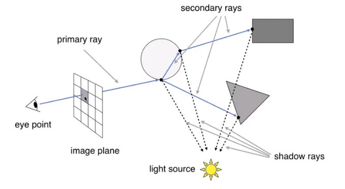
0. Ray-Surface Intersection

   0. Ray Equatiom

      Ray is defined by its origin and a direction vector
      $$
      r(t)=O+t\vec d,0\leq t <\infty
      $$
      where $r$ is int, along ray, $t$ is “time”, $O$ is origin and $\vec t$ is normalized direction.

   1. Ray Intersection With Sphere

      Suppose the equation of sphere is $p:(p-c)^2-R^2=0$， the intersection $p$ must satisfy both equations（ray and sphere）

      Solve for intersection $(O+t\vec d - c)^2-R^2=0$, by using the quadratic formula ,we can get
      $$
      t=\frac {-b\pm \sqrt{b^2-4ac}}{2a}
      $$

   2. Ray Intersection With Implicit Surface

      Firstly, we get a generay implicit surface $p:f(p)=0$

      then substitute ray equation: $f(O+t\vec d)=0$

      Solve the real,postive roots

   3. Ray Intersection With Triangle Mesh（Be careful that the genus should be $0$）

      0. Why?

         0. Rendering: visibility, shadows, lighting …
         1. Geometry: inside/outside test

      1. How?

         0. Simple idea：just intersect ray with each triangle. But it slow.
         1. Note：Can have 0, 1 intersections（ignoring multiple intersections）

         Triangle is a plane, Ray-plane intersection. Test if hit point is inside triangle

      2. Plane Equation

         Plane is defined by normal vector and a point on plane：a normal, $\vec N$, and a point, $p’$, not in the normal. So the equation is
         $$
         p:(p-p’)\cdot \vec N=0 , or \space ax+by+cz+d=0
         $$

      3. Solve for intersection
         $$
         Set\space r=r(t)\\
         (p-p’)\cdot \vec N=(O+td-p’)\cdot \vec N=0\\
         t=\frac {(p’-O)\cdot \vec N}{\vec d \cdot \vec N}\space and \space Check:0\leq t\leq \infty
         $$

   4. Moller Trumbore Algorithm

      A faster approach, giving barycentric coordinate directyly.

      Derivation in the discussion section!（By cramer）
      $$
      \vec O+t\vec D=(1-b_1-b_2)\vec P_0+b_1\vec P_1+b_2\vec P_2\\
      \left[\begin{matrix} t\\b_1\\b_2 \end{matrix}\right]=\frac 1{\vec S_1 \cdot \vec E_1}\left[\begin{matrix} \vec S_2\cdot \vec E_2\\\vec S_1\cdot \vec S\\\vec S_2\cdot \vec D \end{matrix}\right]
      $$
      where
      $$
      \vec E_1=\vec P_1 - \vec P_0\\
      \vec E_2=\vec P_2 - \vec P_0\\
      \vec S=\vec O -\vec P_0\\
      \vec S_1=\vec D \times \vec E_2\\
      \vec S_2=\vec S \times \vec E_1
      $$

   5. Accelerating Ray-Surface Intersection

      0. Simple ray-scene intersection

         Exhaustively test ray-intersection with every objecy and should find the closet hit（with minimum $t$）. The problem：Naive algorithem = pixels $\times$ objects（$\times$ bounces） and it is very slow

   6. Bounding Volume

      Quick way to avoid intersections：bound complex object with a simple volume, which object is fully contained in the volum. It can be easy know that the ray doesn’t hit the volume, it doesn’t hit the object. So test BVol first, then test object if it hits

      0. Ray-Intersection With Box

         Understanding：box is the itersection of 3 pairs of slabs

         Specifically：We often use an Axis-Aligned Bounding Box（AABB）

      1. Ray Intersection with Axis-Aligned Box

         2D example; 3D is the same.

         We compute intersections with slabs and take intersection of $t_{min}/t_{max}$ intervals

         The following picture showed the Intersection with $x$ plane

         

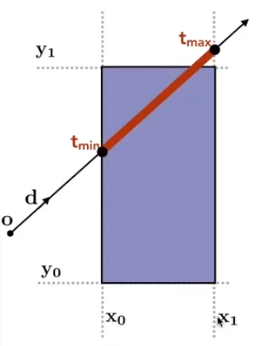
         The following picture showed the Intersection with $y$ plane

         

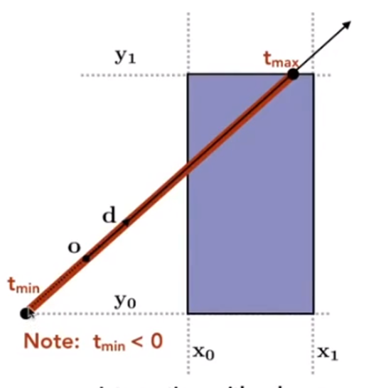
         The following picture showed the Final Intersection result

         

      2. Recall：a box（3D）= three pairs of infintely large slabs

         0. Key ideas：The ray enters the box only when it enters all pairs of slabs and exits the box as long as it exits any pair of slabs.

            For each pair, caculate the $t_{min}$ and $t_{max}$（negative is fine）So, for the 3D box, $t_{enter}=max(t_{min}),t_{exit}=min(t_{max})$

         1. If $t_{enter}<t_{exit}$, we know the ray stays a while in the box（So they must intersect！）（not done yet, see the next slide）

         2. However, ray is not a line, it should check whether $t$ is negative for physical coreectness

         3. What if $t_{exit}<0$? It means that the box is “behind” the ray - no inersection！

         4. What if $t_{exit}\geq 0$ and $t_{enter}< 0$? It means the rays orgin is inside the box - have intersection

         5. In a nutshell, ray and AABB intersect if and only if
            $$
            t_{enter}<t_{exit}\ and \space t_{exit}\geq 0
            $$

      3. Why Axis-Aligned?

         General model, the $t$ we should have 3 subtractions, 6 multiplies and i division; but the slabs perpendicular to x-axis just need 1 subtraction and 1 division（recall the fomula from the foregoing)

      4. Using AABBs to accelerate ray tracing

         0. Uniform grids

            0. Preprocess - Build Acceleration Grid
               0. Find bounding box
               1. Create grid
               2. Store each object in overlapping cells
               3. Step through grid in ray traversal order - For each grid cell：Test intersection with all objects stored at that cell
            1. Grid Resolution
               0. One cell - no spped up
               1. Too many cells - Inefficiency due to extraneous grid traversal
               2. Heuristic - cells = $C\times objs$ ,$C\approx 27$ in 3D
            2. When They Work Well on large collection of objects that are distributed evenly in size and space
            3. When they Fail that “Teapot in a stadium” problem

         1. Spatial Partitions - example by KD-Tree

            

            

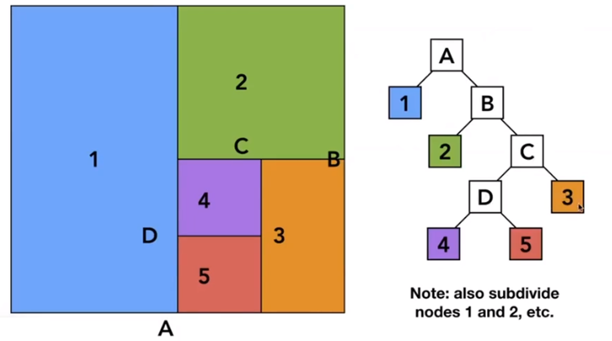
            0. Bilud: Internal nodes store

               0. Split axis: $x,y$ or $z$ axis
               1. Split position: coordinate of split plane along axis
               2. childrenL pointers to child nodes
               3. No ovjects are stored in internal nodes
               4. Leaf nodes store list of objects

            1. Traversing a KD-Tree

               If the ray have intersect with the leaf node, the program will check whether the ray intersect with all objects.

         2. Object Partitions - Volume Hierarchy（BVH）

            

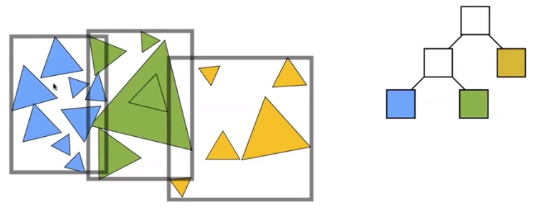
            Find bounding box, then recursively split set of objects in two subsets. Then recompute the bounding box of the subsets.

            Stop when necessary and store objects in each leaf node

            0. Building

               0. Choose a dimension to split

               1. Heuristic #1： Always choose the longest axis in node

                  ​ #2：Split node at location of median object（keep balance）

                  Be careful that in a random sequence, if you want to find the $n-th$ number, it just need $O(n)$

               2. Termination criteria: stop when node contains few elements

            1. BVH Traversal’s’ pseudocode

               Intersect(Ray ray, BVH node){
                   if (ray misses node.bbox) return;
                   if (node is a leaf node)
                       test intersection with all objs;
                       return closeest intersection;
               
                   hit1 = Intersect(ray, node.childl);
                   hit2 = Intersect(ray, node.childr);
               
                   return the closer of hit1, hit2;
               } 

         3. Spatial vs Object Partions

            0. Spatial
               0. Partition space into non-overlapping regions
               1. An object can be contained in multiple regions
            1. Object partition
               0. Partition set of objects into disjoint subsets
               1. Bounding boxes fore each set may overlap in space

Basic radiometry

Advertisement：new topic from now on, scarcely covered in other graphics courses

0. Motivation

   In assignment 3, we implement the Blinn-Phong model. The light intensity $I=10$ for example, but what is $10$? But the Whitted style ray tracing doesn’t give you CORRECT results if just “$I=10$”

   All the answers can be found in radiometry

1. Radiometry

   Measurement system and units for illumination. And it can accurately measure the spatial properties of light. The radiometry can perform lighting calculations in a physically correct manner

   0. Radiant flux

      0. Radiant Energy - the energy of electromagenetic radiation. It is measured in units of joules, and denoted by the symbol：$Q[J=Joule]$

      1. Radiant flux（power） is the ennergy emitted, reflected, trransmitted or received, per unit time
         $$
         \Phi \equiv\frac {dQ}{dt}[W=Watt][lm=lumen]
         $$

   1. Intensity

      0. The radiant （luminous） intensity is the power per unit solid angle（立体角） emitted by a point light source
         $$
         I(\omega)\equiv\frac {d\Phi}{d\omega}[\frac W{sr}][\frac {lm}{sr}=cd=candela]
         $$
         The candela is one of the seven SI base units

      1. Angles and Solid Angles

         0. Angles：ratio of subtended arc length on circle to radius $\theta = \frac lr$, circle has $2 \pi$ radians

         1. Solid angle：ratio of subtended area on sphere to radius squared $\Omega=\frac A{r^2}$, sphere has $4\pi$ steradians

         2. Differential Solid Angles：

            $dA=(rd\theta)(d\sin\theta d\phi)=r^2\sin\theta d\theta d\phi$

            $d\omega=\frac {dA}{r^2}=\sin\theta d\theta d\phi$

            $\Omega=\int_{S^2}d\omega=\int_0^{2\pi}\int_0^{\pi}\sin\theta d\theta d\phi=4\pi$

         3. $\omega$ as a direction vector

         4. Isotropic Point Source
            $$
            \Phi c= \int_{S^2}Id\omega=4\pi I,then\space I=\frac {\Phi}{4\pi}
            $$

   2. Irradiance

      The irradiance is the power per（perpendicular/projected） unit area incident on a surface point
      $$
      E(x)\equiv\frac {d\Phi(x)}{dA}[\frac W{m^2}][\frac {lm}{m^2}=lux]
      $$
      Review Lambert’s Cosine Law, the irradiance at surface is proportional to cosine of angle between light direction and surface normal

      Correction：Irradiance Falloff

      Assume light is emitting power $\Phi$ in a uniform angular distributition, Compare irradiance st surface of two shperes:

      0. $r=1:E=\frac {\Phi}{4\pi}$
      1. $r=x$：$E’=\frac {\Phi}{4\pi r^2}=\frac E{r^2}$

   3. Radiance

      Radiance is the fundamental field quantity that describes the distribution of light in an environment

      0. Radiance is the quantity associated with a ray
      1. Rendering is all about computin radiance

      The radiance （luminance）is the power emitted, reflected, transmitted or received by a surfac, per unit solid angle, per projected unit area

      
      $$
      L(p,\omega)\equiv \frac {d^2\Phi(p,\omega)}{d\omega dA\cos \theta}[\frac W{sr \space m^2}][\frac {cd}{m^2}=\frac{lm}{sr\space m^2}=nit]
      $$
      where $\cos \theta$ account for projected surface area

      Recall

      0. Irradiance ：power per projected unit area
      1. Intensity：power per solid angle

      So

      0. Radiance ：Irradiance per solid angle
      1. Radiance ：Intensity per projected unit area

   4. Irradiance vs. Radiance

      Irradiance：total power received by area $dA$

      Radiance：power ceceived by area $dA$ from “direction” $d\omega$

      and we have $H^2$ is a unit Hemisphere
      $$
      dE(p,\omega)=L_i(p,\omega)\cos\theta d\omega\\
      E(p)=\int_{H^2}L_i(p,\omega)\cos \theta d\omega
      $$

2. Bidirectional Reflectance Distribution Function（双向反射分布函数：BRDF）

   0. Reflection at a Point

      

      Radiance from direction $\omega_i$ turns into the power $E$ that $dA$ receives, then power $E$ will become the radiance to any other direction $\omega_i$

      The differential irradiance incoming is $dE(\omega_i)=L(\omega_i)\cos\theta_id\omega_i$, the differential radiance exiting （due to $dE(\omega_i)$）： $dL_r(\omega_r)$

   1. BRDF’s Definetion

      

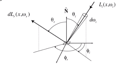
      The Bidirectional Reflectance Distribution Function（BRDF） represents how much light is reflected into each outgoing direction $\omega_r$ from each incoming direction
      $$
      f_r(\omega_i \rightarrow \omega_r)=\frac {dL_r(\omega_r)}{dE_i(\omega_i)}=\frac{dL_r(\omega_r)}{L_i(\omega_i)\cos\theta_id\omega_i }[\frac1{sr}]
      $$
      Emit the mathematical and physical analysis, the BRDF is illustrate the interact object with the light,. So it can determine the material of the object.

   2. The Reflection Equation:
      $$
      L_r(p,\omega_r)=\int_{H^2}f_r(p,\omega_i \rightarrow\omega_r)L_i(p,\omega_i)\cos\theta_id\omega_i
      $$

   3. Recursive Equation

      Reflected radiance depends on incoming radiance, but incoming radiance depends on reflected radiance（at another point in the scene）

   4. The Rendering Equation

      Re-write the reflection equation
      $$
      L_r(p,\omega_r)=\int_{H^2}f_r(p,\omega_i \rightarrow\omega_r)L_i(p,\omega_i)\cos\theta_id\omega_i
      $$
      by adding an Emission term to make it general. So the Rendering Equation is
      $$
      L_o(p,\omega_o)=L_e(p,\omega_o)+\int_{\Omega^+}L_i(p,\omega_i)f_r(p,\omega_i,\omega_o)(n\cdot\omega_i)d\omega_i
      $$
      Node that we assume that all directions are pointing outwards now

   5. Reflection Equation

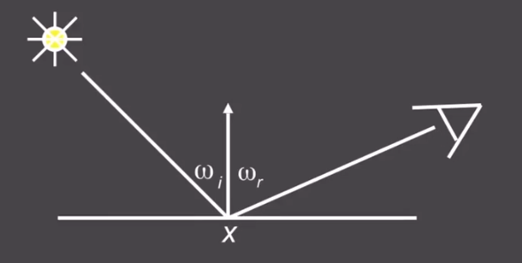      $$ L_r(x,\omega_r)=L_e(x,\omega_r)+L_i(x,\omega_i)f(x,\omega_i,\omega_r)(\omega_i.n) $$ Where $L_r$ is Reflected Light（output image）, $L_e$ is Emiision, $L_i$ is incident light (from light source) , $(\omega_i,n)$ is cosine of incident angel and $f$ is BRDF, then we add some extra light source

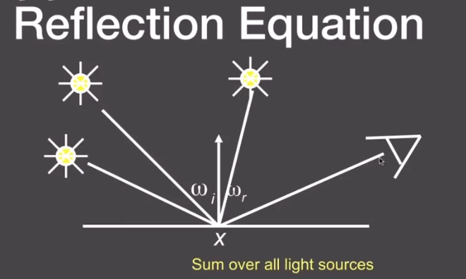
      the Equation now change to
      $$
      L_r(x,\omega_r)=L_e(x,\omega_r)+\sum L_i(x,\omega_i)f(x,\omega_i,\omega_r)(\omega_i.n)
      $$
      Then change an area to light source area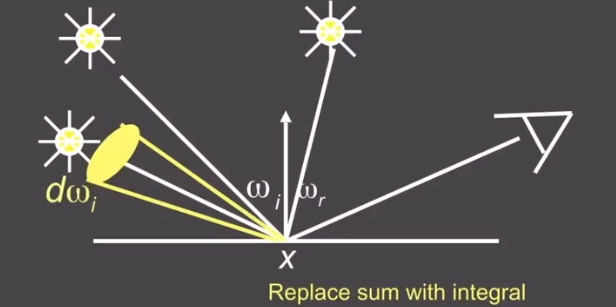

      

      the equation change to
      $$
      L_r(x,\omega_r)=L_e(x,\omega_r)+\int_{\Omega} L_i(x,\omega_i)f(x,\omega_i,\omega_r)(\omega_i.n)d\omega_i
      $$
      But some of light comes from other object by reflecting, so the pic would change

      

      and the equation becomes to
      $$
      L_r(X,\omega_r)=L_e(X,\omega_r)+\int_{\Omega} L_r(X’,-\omega_i)f(x,\omega_i,\omega_r)(\omega_i.n)d\omega_i
      $$
      where $L_r$ there is reflected light.

   6. Rendering Equation as Intergral Equation
      $$
      L_r(X,\omega_r)=L_e(X,\omega_r)+\int_{\Omega} L_r(X’,-\omega_i)f(x,\omega_i,\omega_r)(\omega_i.n)d\omega_i
      $$
      is a Fredholm Intergral Equation of second kind [extensively studied numerically] with canonical form
      $$
      L(u)=e (u)+\int L(v)K(u,v)dv
      $$
      even we can write it as linear operator equation
      $$
      l(u)=e(u)+\int l(v)K(u,v)dv
      $$
      where $K(u,v)$ is kernel of equation Light transport operator, and it can be write as
      $$
      L=E+KL
      $$
      It can be sicretized to a simple matrix equation[or system of simultaneous linear equations]（$L$,$E$ are vectors, $K$ is the light transport matrix）. Then it can general class numberucak Monte Carlo methids and approximate set of all paths of light in scene
      $$
      L=E+KL\\IL-KL=E\\(I-K)=E\\L=(I-K)^{-1}E
      $$
      According to binomia theorem（二项式定理）
      $$
      L=(I+K+K^2+K^3+…)E\\L=E+KE+K^2E+K^3E+…
      $$
      then the $E$s of last equation, from the left to right, we can illustrate them ase Emission directly from light sources, direct illumination on surfaces, indirect illumiantion（one bounce indirect[Mirrors, Refraction]） and Twoi bounce indirect illumation and etc.

      We can shading in rasterization on $E$ and $KE$, but the follows are hard to shade

Probability Review

Review some easy probability knowledge which will use in the following content

0. Random Variables

   $X$：random variable. Represents a distribution of potential values

   $X\sim p(x)$：probability density function（PDF）. Describles relative probability of a random process choosing value $x$

1. Probabilities

   n discrete value $x_i$, With probability $p_i$, Requirements of a probability distribution：$p_i\geq0$, $\sum p_i=1$

2. Expected Value of a Random Variable

   The average value that one obtains if repeatedly drawing samples from the random distribution. $X$drawn from distribution with $n$ discrete values $x_i$ with probabilities $p_i$, the expected value of $X: E(x)=\sum x_ip_i$

3. Continuous Case： Probability Distribution Function（PDF)

   A random variable $X$ that can take any of a continuos set of values. where the relative probability of a particular value is given by a continuous probability density function $p(x)$.

   Condition on $p(x)\geq0\ and\ \int p(x)dx=1$

   Expected value of $X：E(X)=\int xp(x)dx$

4. Function of a Random Variable

   A function $Y$ of a random variabvle $X$ is also a random variable: $X\sim p(x)$ and $Y=f(X)$, the expected value oif a function of a random variable $E(Y)=E(f(x))=\int f(x)p(x)dx$

5. Monte Carlo Intergration

   Why：We want to solve an intergral, but it can be too difficult to solve annalyticcally

   How：estimate the integral of a function by averraging random samples of the function’s value

   0. Some definetion of it

      0. Deinite integral： $\int_a^bf(x)dx$
      1. Random variable：$X_i\sim p(x)$

      Then the Monte Carlo estimator is
      $$
      F_N=\frac 1N\displaystyle\sum_{i=1}^N\frac {f(X_i)}{p(X_i)}
      $$

   1. Example Uniform Monte Carlo Estimator

      Assume $f(x)=C$

      0. Deinite integral： $\int_a^bf(x)dx$

      1. Uniform Random variable：$X_i\sim p(x)=\frac 1{b-a}$

      Then the basic Monte Carlo estimator
      $$
      F_N=\frac {b-a}N\displaystyle\sum_{i=1}^Nf(X_i)
      $$

   2. Some notes

      0. The more samples, the less variance
      1. Sample on $x$, intergrate on $x$

Path Tracing

0. Motibation：Whitted-Style Ray Tracing

   0. Whitted-style ray tracing：

      0. Always perform specular reflections / refractions
      1. Stop bouncing at diffuse surfaces

      But it may not reasonable , so let’s progressively improve upon Whitted-Style Ray Tracing and lead to our path tracing algorithm!

   1. Problem of Whitted-Style Ray Tracing

      0. Glossy reflection
      1. Diffuse materials

   2. So it seems that Whitted-Style ray tracing is Wrong, but the rendering equation is corret

      But it involves：Solving an integral over the hemisphere and recursive execution

1. A Simple Monte Carlo Solution

   Suppose we want to render one pixle（point）in the followingf scene for direct illumination only

   

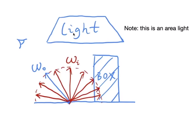
   Abuse the concept of Reflection Equation a little bit
   $$
   L_o(p,\omega_o)=\int_{\Omega^+}L_i(p_i,\omega_i)f_r(p,\omega_i,\omega_o)( n\cdot \omega_i)d\omega_i
   $$
   Note again that we assume all direction are pointing outwards. Fancy as it is , it’s still just an integration over directions. So, of course, we can solve it using Monte Carlo integration.

   We want to comput the radiance at $p$ towards the camera
   $$
   L_o(p,\omega_o)=\int_{\Omega^+}L_i(p_i,\omega_i)f_r(p,\omega_i,\omega_o)( n\cdot \omega_i)d\omega_i\\
   \int_a^bf(x)dx\approx\frac 1N\displaystyle\sum_{i=1}^N\frac {f(X_i)}{pdf(X_i)}\ X_k\sim p(x)
   $$

   $$
   f(x)=L_i(p_i,\omega_i)f_r(p,\omega_i,\omega_o)( n\cdot \omega_i)
   $$

   So, what’s our PDF?

   We assume uniformly sampling the hemisphere, the PDF is $p(\omega_i)=\frac 1{2\pi}$

   So, in general
   $$
   L_o(p,\omega_o)=\int_{\Omega^+}L_i(p_i,\omega_i)f_r(p,\omega_i,\omega_o)( n\cdot \omega_i)d\omega_i
   \\\approx \frac 1N\displaystyle\sum_{i=1}^N\frac{L_i(p_i,\omega_i)f_r(p,\omega_i,\omega_o)( n\cdot \omega_i)}{pdf(\omega_i)}
   $$
   Note abuse notation a little bit for $i$

   Then we will write pseudocode

   shade(p, wo)
       Randomly choose N direcytions wi~pdf
       L0 = 0.0
       For each wi
           Trace a ray r(p,wi)
           If ray r hit the light
               Lo += ( 1 / N ) * L_i * f_r * cosine / pdf(wi)
       return Lo

2. Introduction Global Illumination

   0. One more step forwad - What if a ray hits an object?

      

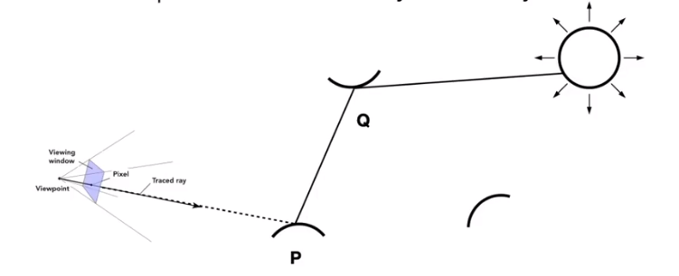
      We can know that $Q$ also reflects light to $P$.

      How much? The dir.illum. at Q

      So the pseudocode can revise

      shade(p, wo)
          Randomly choose N direcytions wi~pdf
          L0 = 0.0
          For each wi
              Trace a ray r(p,wi)
              If ray r hit the light
                  Lo += ( 1 / N ) * L_i * f_r * cosine / pdf(wi)
              //new here
              Else If ray r hit an object at q
                  Lo += ( 1 / N ) * shade(q, -wi) * f_r * cosine / pdf(wi)
          return Lo

      But we doesn’t sovle it. Because

      0. Explosion of rays as bounces go up：$num_{RAY}=N^{bounces}$

         We observation：rays will not explode if and only if $N=1$, So the

         shade(p, wo)
             Randomly choose only ONE direcytions wi~pdf
             Trace a ray r(p,wi)
             If ray r hit the light
                 return L_i * f_r * cosine / pdf(wi)
             Else If ray r hit an object at q
                 return shade(q, -wi) * f_r * cosine / pdf(wi)

         This is path tracing! （FYI, Distributed Ray Tracing if N != $1$）

      1. Ray Generation

         Maybe some readers will think that this will be nosiy! But don’t be worry, just trace more paths through each pixel and average their radiance

         

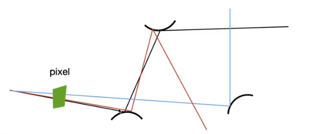
         Then, about this ,it is very similar to ray casting in ray tracing

         ray_ generation (camPos, pixel)
             Uniformly choose N sample positions within the pixel
             pixel_ radiance = 0.0
             For each sample in the pixel
                 Shoot a ray r(camPos, cam_ to_ sample)
                 If ray r hit the scene at p
                     pixel_ radiance += 1 / N * shade(P, sample_to cam)
                 Return pixel_ radiance    

      2. Path Tracing

         But their have some other problems in shade()？The recursive algorithm will never stop!

         Dilemma: the light does not strop bouncing indeed

         Cutting #bounces == cutting energy

         Solution：Russian Roulette（RR）- all about probability

         ​ With probability $0<P<1$, you are fine

         ​ With probability $1-P$, otherwise

         Previously, we always shoot a ray at a shading point and get the shading result $L_o$, suppose we manually set a probability $P(0<P<1)$

         With probability $P$, shoot a ray and return the **shading result divided by P：$L_o/P$

         With probability $1-P$, don’t shoot a ray and you’ll get 0

         In this way, you can still expect to get $L_o$：$E=P\times(\frac {L_o}{P}+(1-P)\times 0)=L_o$

         Now we revise the API

         shade(p, wo)
             Manually specify a probability P_RR
             Randomly select ksi in a uniform dist. in[0,1]
             If (ksi>P_RR) return 0.0;
         
             Randomly choose only ONE direcytions wi~pdf
             Trace a ray r(p,wi)
             If ray r hit the light
                 return L_i * f_r * cosine / pdf(wi) / P_RR
             Else If ray r hit an object at q
                 return shade(q, -wi) * f_r * cosine / pdf(wi) / P_RR

      3. Path Tracing

         Now we already have a correct version of path tracing, but it’s not really efficient. The lower samples per pixel（SPP） , the more noisy . Before we make it better, we shoule understand the reason of being inefficient.

         0. Sampling the Light

            Consider the same point, the volume of the light source will change. In one case, only 5 rays can meet the light. But in the specail case that 50,000 rays but only one meet the light.

            In the latter, a lot of rays are “wasted”, if we uniformly sample the hemisphere at the shading point.

         1. Pure math method

            Monte Carlo methods allows any sampling methods, so we can sample the light（therefore no rays are “wasted”）

            Assume uniformly sampling on the light, $pdf=\frac 1A$, beacuse $\int pdf dA=1$

            

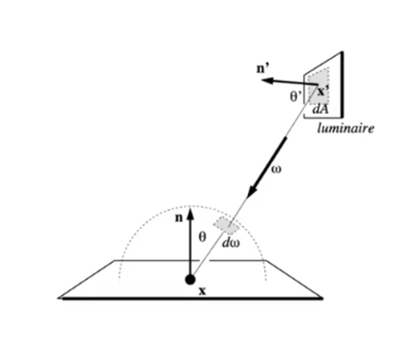
            But the rendering equation intergrates on the solid angle:$L_o=\int L_ifr \cos\theta d\omega$

            Recall Monte Carlo Intergration：sample on $x$ & integrate on $x$.

            We change it to sapmle on $dA$ and intergral of $A$, which we just need the relationship between $d\omega$ and $dA$.

            Acoording to the picture above, we can easy get that
            $$
            d\omega=\frac {dA\cos \theta ’}{||x’-x||^2}
            $$
            Note the $\theta ‘$ not the $\theta$, then rewrite the rendering equation as
            $$
            L_o(x,\omega)=\int _A L_i(x,\omega_i)f_r(x,\omega_i,\omega_o)\frac {\cos \theta\cos \theta ’}{||x’-x||^2}dA
            $$
            Now an intergration on the light ! Monte Carlo intergration：$f(x)$ everything inside $pdf :\frac 1A$

         2. What’s more

            Previously, we assume the light is “accidentally” shot by uniform hemisphere sampling

            Now we consider the radiance coming from two parts

            0. light source （direct, no need to have RR）
            1. other reflections（indirect, RR）

            shade(p,wo)
                # contribution from the light source
                Uniformly sample the light at x'' (pdf_light = 1 / A)               
                L_dir = L_i * f_r * cos θ * cos θ''  |x'' - p|^2 / pdf_light
            
                # contribution from other reflectors
                L_indir = 0.0
                Test Russian Roulette with probability P_RR
                Uniformly sample the hemisphere toward wi (pdf_hemi = 1 /2pi)
                Trace a ray r(p, wi)
                if ray r hit a non-emmiting object at q
                    L_indir =  shade (q,-wi)=f_r * cos θ /pdf_hemi/ P_RR
                Return L_dir + L_indir

         3. At last

            One final thing：how do we know if the sample on the light is not blocked or not？

            Just revise the shade a little

            L_dir = 0.0
            Uniformly sample the light at x'' (pdf_light = 1 / A) 
            shoot a ray from p to x''
            if the ray is not blocked in the middle
                L_dir =....

   1. Some Side Notes

      0. Consider if the most challenging in undergrad CS
      1. Why? Physic, probability, calculus, coding
      2. Learning PT will help you understand deeper in these

      Maybe the PT is not “introduction”, but it’s modern. And learning it will be rewarding also because it is almost 100% correct.

   2. Ray tracing ： Previous vs. Modern Concepts

      Previous ：Ray tracing == Whitted-style ray tracing

      Modern：The general solution of light transport, include （Unidirectional & bidirectional）path tracing, photon mapping（光子映射）, Metropolis light transport ,VCM/UPBP and etc

   3. Something hasn’t covered / won’t cover

      0. Uniformly sampling the hemisphere
      1. Monte Carlo integration allows arbitrary pdfs - important sampling
      2. Random numbers matter - low discrepancy sequences
      3. can combine sample the hemisphere and the light - multiple imp.samplig
      4. The radiance of a pixel is the average of radiance on all paths passing through it - pixel reconstruction filter
      5. The radiance of a pixel isn’t the color of a pixel - gamma correction, curves, color space

6. Materials and Appearances

What is Material in Computer Graphics?

Material == BRDF!

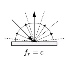
0. Diffuse / Lambertian Material：

1. Light is equally reflected in each output direction. Suppose the incident lighting is uniform

   

$$
L_o(\omega_o)=\int_{H^2}f_rL_i(\omega_i)\cos\theta_id\omega_i\\
=f_rL_i\int_{H^2}\cos\theta_id\omega_i\\
=\pi f_rL_i\\
f_r=\frac \rho \pi
$$

1. Glossy material（BRDF）

   Ideal reflective / refractive material（BSDF*）

   Perfect Specular Reflection

   

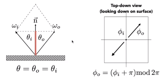
   and then
   $$
   \omega _o+\omega _i=2\cos\theta \vec n = 2(\omega \cdot \vec n)\vec n\\
   \omega _o=-\omega _i+2(\omega _i\cdot \vec n)\vec n
   $$

2. Specular Refraction

   In addition to reflecting off surface, light may be transmitted through surface.

   Light refracts when it enters a new medium. （Ocean：caustics)

   Snell’s Law

   Transmitted angle depends on

   0. index of refraction （IOR） for incident ray

   1. index of refraction （IOR） for exiting ray
      $$
      \eta_i\sin\theta_i=\eta_t\sin\theta_t\\
      \phi_t=\phi_i\pm \pi
      $$

   Law of Refraction
   $$
   \cos\theta_t=\sqrt {1-(\frac {\eta_i}{\eta_t})^2(1-\cos^2\theta)i}
   $$
   Total internal reflection

   When light is moving from a more optically dense medium to a less optically dense medium $\eta_i /\eta_t>1$

   Light incident on boundary from large enough angle will not exit medium

   Fresnel Reflection / Term

   Reflectance depends on incident angle（and polarization of light）

   The formulae of it are
   $$
   R_s=\left|\frac {n_1\cos\theta_i-n_2\cos\theta_t}{n_1\cos\theta_i+n_2\cos\theta_t}\right|^2=\left|\frac {n_1\cos\theta_i-n_2 \sqrt {1-(\frac {\eta_1}{\eta_2})^2(1-\cos^2\theta})}{n_1\cos\theta_i+n_2\sqrt {1-(\frac{\eta_1}{\eta_2})^2(1-\cos^2\theta})} \right|^2\\R_p=\left|\frac {n_1\cos\theta_t-n_2\cos\theta_i}{n_1\cos\theta_t+n_2\cos\theta_i} \right|^2=\left|\frac{n_1\sqrt {1-(\frac {\eta_1}{\eta_2})^2(1-\cos^2\theta_i)}-n_2\cos\theta_t}{n_1\sqrt {1-(\frac {\eta_1}{\eta_2})^2(1-\cos^2\theta_i)}+n_2\cos\theta_t} \right|^2\\R_{eff}=\frac 12(R_s+R_p)
   $$

It’s too difficult, there is an approximate - Schlick’s approximation $R(\theta)=R_0+(1-R_0)(1-\cos\theta)^5\ ,\ R_0=(\frac {n_1-n_2}{n_1+n_2})$

Microfacet Material

Microfacet Theory

0. Rough surface - Macroscale is flat & rough and microscale is bumpy & specular

1. Individual elements of surface act like mirrors

   Known as Microfacets and each microfacet has its own normal

2. Microfacet BRDF

   Key：the distribution of microfacets’ normals

   0. Concentrated <==> glossy
   1. Spread <==> diffuse

   The formula

   
   $$
   f(i,o)=\frac {F(i,h)G(i,o,h)D(h)}{4(n,i)(n,o)}
   $$
   where $F$ is Fresnel term, $G$ is shadowing-masking term and the $D$ is distribution of normals

Isotropic / Anisotropic Materials（BRDFs） 各向同性和各向异性

Key: directionality of underlying surface

Anisotropic BRDFs: Reflection depends on azimuthal angle $\phi$ $f_r(\theta_i,\phi_i,\theta_r,\phi_r)\neq f_r(\theta_i,\theta_r,\phi_r-\phi_i)$

Results from oriented microstructure of surface.

3. Properties of BRDFs

   0. Non-negativity: $f_r(\omega_i\rightarrow\omega_r)\geq0$

   1. Linearity: $L_r(p,\omega_r)=\int_{H^2}f_r(p,\omega_i\rightarrow\omega_r)L_i(p,\omega_i)\cos\theta_id\omega_i$

   2. Reciprocity principle: $f_r(\omega_r\rightarrow\omega_i)=f_r(\omega_i\rightarrow\omega_r)$

   3. Energy conservation:$\forall\omega_r\int_{H^2}f_r(\omega_i\rightarrow\omega_r)\cos\theta_id\omega_i\leq1$

   4. Isotropic vs. anisotropic

      If isotropic $f_r(\theta_i,\phi_i,\theta_r,\phi_r)= f_r(\theta_i,\theta_r,\phi_r-\phi_i)$ .

      Then from reciprocity $f_r(\theta_i,\theta_r,\phi_r-\phi_i)=f_r(\theta_i,\theta_r,\phi_i-\phi_r)=f_r(\theta_i,\theta_r,|\phi_r-\phi_i|)$

4. Measuring BRDFs

   0. Motivation:

      Avoid need to develop / derive model - Automatically includes all of the scattering effects present

      Can accurately render with real-world materials - Useful for product design, special effects …

   1. Image-Based Measurement

      

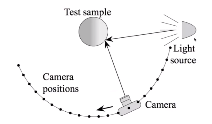
   2. General approach

      for each outgoing direction wo
          move light to illuminate surface with a thin beam from wo
          for each incoming direction wi 
              move sencor to be at direction wi from surface
              measure incident radiance

   3. Improving efficiency

      0. Isotropic surfaces reduce dimensionality from 4D to 3D
      1. Reciprocity reduces # of measurements by half
      2. Clever optical systems

   4. Representing Measured BRDFs

      0. Compact representation

      1. Accurate representation of measured data

      2. Efficient evaluation for arbitrary pairs of directions

      3. Good distributions available for importance sampling

      4. Tabular Representation - store regularly-spaced samples in $(\theta_i,\theta_o,|\phi_i-\phi_o|)$（Better: reparameterize angles to better match specularities）

         Generally need to resample measured values to table. But it have very high storage requirements

7. Advanced Topics in rendering

Advanced Light Transport

0. Biased vs. Unbiased Monte Carlo Estimators

   0. An unbiased Monte Carlo technique does not have any systematic error

      The expected value of an unbiased estimator will always be the correct value, no matter how many samples are used

   1. Otherwise, biased

      One special case, the expected value converges to the correct value as infinite #samples are used - consistent

1. Unbiased light transport methods

   1. Bidirectional path tracing（BDPT）

      0. Recall: a path connects the camera and the light
      1. BDPT
         0. Traces sub-paths from both the camera and the light
         1. Connects the end points from both sub-paths
         2. Suitable if the light transport is complex on the light’s side
         3. Difficult to implement & quite slow

   2. Metropolis light transport （MLT）

      0. Idea: Jumping from the current sample to the next with some PDF

      1. It is good at locally exploring difficult light paths

      2. Key: Locally perturb an existing path to get a new path

         

      3. It works great with difficult light paths but also unbiased

      4. Disadvantage

         0. Difficult to estimate the convergence rate
         1. Does not guarantee equal convergence rate per pixel
         2. So usually produces “dirty” results
         3. Therefore, usually not used to render animations

2. Biased light transport methods

   1. Photon Mapping

      A biased approach & a two-stage method and very good at handling Specular-Diffuse-Specular(SDS) paths and generating caustics

      Stage 0 - photon tracing

      Emitting photons from the light source, bouncing them around, then recording photons on diffuse surfaces

      Stage 1 - photon collection ( final gathering)

      Shoot sub-paths from the camera, bouncing them around, until they hit diffuse surfaces

      Calculation - local density estimation

      idea: area with more photons should be brighter

      For each shading point, find the nearest $N$ photons. Take the surface area that over

      Why biased?

      Because local Density estimation
      $$
      \frac {dN}{dA}\neq\frac{\Delta N}{\Delta A}
      $$
      But in the sense of limit, more photons emitted ->The same $N$ photos covers a smaller $\Delta A$ , and the $\Delta A$ is closer to $dA$. So, biased but consistent.

      An easier understanding bias in rendering

      Biased == blurry and consistent == not blurry with infinite #samples

      *not do a “const range” *

   2. Vertex connection and merging

      A combination of BDPT and Photon Mapping

      Key idea

      Let’s not waste the sub-paths in BDPT if their end points cannot be connected but can be merged and use photon mapping to handle the merging of nearby “photons”

3. Instant radiosity （VPL / many light methods）

   Sometimes also called many-light approaches

   Key idea: Lit surfaces can be treated as light sources

   Approach: Shoot light sub-paths and assume the end point of each sub-path is a Virtual Point Light (VPL), then render the scene as usual using these VPLs .

   Pro fast and usually gibes good results on diffuse scenes

   Cons Spikes will emerge when VPLs are close to shading points and cannot handle glossy materials

Advanced Appearance Modeling

0. Non-surface models

   Such like cloud or fog, at any point as light travels through a participating medium, it can be （partially） absorbed and scattered.

   0. Participating media

      Use Phase Function to describe the angular distribution of light scattering at any point $x$ with participating media.

      Rendering

      0. Randomly choose a direction to bounce
      1. Randomly choose a distance to go straight
      2. At each ‘shading pointy’, connect to the light

   1. Hair / fur / fiber（BCSDF）

      0. Kajiaya-Kay Model
      

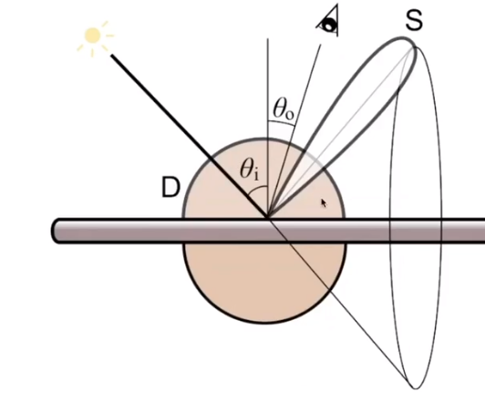
      1. Marschner Model

         

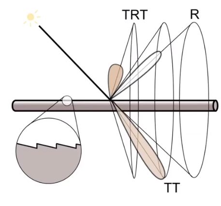
         Glass-like cylinder: 3 types of light interactions: R, TT, TRT （reflection = R, transmission =T ）

         2. Fur - Double Cylinder Model - Lobes
         

   2. Granular material（颗粒材质）

      With procedural definition, we can avoid explicit modeling of all granules

1. Surface models

   0. Translucent material (BSSRDF)

      Subsurface Scattering - Visual characteristics of many surfaces caused by light exiting at different points than it enters which violates a fundamental assumption of the BRDF.

      BSSRDF: generalization of BRDF; exitant radiance at one point due to incident differential irradiance at another point: $S(x_i,\omega_i,x_o,\omega_o)$

      Generalization of rendering equation: integrating over all points on the surface and all directions
      $$
      L(x_o,\omega_o)=\int_A \int_{H^2} (x_i,\omega_i,x_o,\omega_o)L_i(x_i,\omega_i)\cos \theta_id\omega_idA
      $$
      Dipole Approximation - Approximate light diffusion by introducing two points sources.

   1. cloth

      A collection of twisted fibers

      Given the weaving pattern, calculate the overall behavior and render using a BRDF.

      Render as Participating Media

      Properties of individual fibers & their distribution -> scattering parameters, render as a participating medium

      Render as Actual Fibers

   2. Detailed material （non-statistical BRDF）

      Difficult Path sampling problem

      Solution BRDF over a pixel

      p-NDFs have sharp features

2. Procedural appearance - We can define details without textures by computing a noise function on the fly. 3D noise -> internal structure if cut or broken

   if noise(x, y, z) > threshold reflectance = 1
   else reflectance = 0;

   complex noise function can be very powerful, such like mountain, ocean sea face of wood texture.

8. Cameras, Lenses and Light Fields

Imaging = Synthesis +Capture. but how to capture? By cameras!

Pinholes & Lenses Form Image on Sensor

0. Composition

   0. shutter: exposes sensor for precise duration
   1. Sensor Accumulates irradiance during exposure

1. Why Not Sensors Without Lense

   Each sensor point would integrate light all points on the object, so all pixel values would be similar.

Field of View（FOV）视场

0. Effect of Focal Length on FOV

   

   for a fixed sensor size, decreasing the focal length increases the field of view.
   $$
   FOV = 2\arctan(\frac h{2f})
   $$

1. Focal Length v. Field of View

   0. For historical reasons, it is common to refer to angular field of view by focal length of a lens used on a 35mm-format film （36 x 24mm）
   1. Careful! When we say current cell phones have approximately 28mm “equivalent” focal length, this uses the above convention.

2. To maintain FOV, decrease focal length of lens in proportion to width/height of sensor

Exposure

0. Basic

   0. $H=T\times E$
   1. Exposure = time $\times$ irradiance
   2. Exposure time $T$ - Controlled by shutter
   3. Irradiance $E$
      0. Power of light falling on a unit area of sensor
      1. Controlled by lens aperture and focal length

1. Exposure Controls in Photography

   0. Aperture size

      Change the f-stop by opening / closing the aperture （if camera has iris control）

   1. Shutter speed

      0. Definition:

         Change the duration the sensor pixels integrate light

      1. Side Effect of Shutter Speed:

         0. Motion blur: handshake, subject movement - Doubling shutter time doubles motion blur
         1. Rolling shutter: different parts of photo taken at different times

   2. ISO gain （感光度）

      Change the amplification（analog and/or digital）between sensor values and digital image values

2. ISO(Gain)

   Third variable for exposure;

   Film: trade sensitivity for grain

   Digital: trade sensitivity for noise

      0. Multiply signal before analog-to-digital conversion
            1. Linear effect （ISO 200 needs half the light as ISO 100）

3. F-Number（F-stop）: Exposure Levels

   Written as FN or F/N. N is the f-number, the understanding is that the inverse-diameter of a round aperture

4. Constant Exposure: F-Stop vs Shutter Speed

   If the exposure is too bright/dark, may need to adjust f-stop and/or shutter up/down.

   Photographers must trade off depth of field（景深） and motion blur for moving subjects

5. High-Speed Photography

   Normal exposure = extremely fast shutter speed $\times$（large aperture and/or high ISO）

6. Long-Exposure Photography

Thin Lens Approximation

We just illustrate the ideal thin lens - focal point, and there have 3 properties

a. All parallel rays entering a lens pass through its focal point

b. All rays through a focal point will be in parallel after passing the lens.

c. Focal length can be arbitrarily changed

0. The Thin Lens Equation

   $$ \frac 1f=\frac 1{z_i}+\frac 1{z_o} $$

1. Defocus Blur

   0. Circle of Confusion（CoC）Size

      

      Circle of confusion is proportional to the size of the aperture because of
      $$
      \frac CA=\frac {d’}{z_i}=\frac {|z_s-z_i|}{z_i}
      $$

   1. CoC vs. Aperture Size

      0. Revisiting F-Number

         0. Formal definition: The f-number of a lens is defined as the focal length divided by the diameter of the aperture
         1. Common f-stops on real lenses: 1.4,2, 2.8, 4.0, 5.6, 8, 11, 16, 22, 32
         2. An f-stop of 2 is sometimes written f/2, reflecting the fact that the absolute aperture diameter (A) can be computed by dividing focal length (f) by the relative aperture (N).

      1. Size of CoC is inversely Proportional to F-stop
         $$
         C=A\frac {|z_s-z_i|}{z_i}=\frac fN\frac {|z_s-z_i|}{z_i}
         $$

   2. Ray Tracing ideal Thin Lenses

      

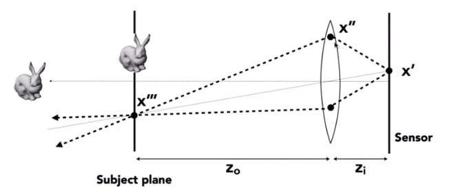
      0. （One possible）Setup:

         0. Choose sensor size, lens focal length and aperture size

         1. Choose depth of subject of interest $z_o$

         2. Calculate corresponding depth of sensor $z$; from thin lens equation（focusing）

      1. Rendering

         0. For each pixel x’ on the sensor （actually film）
         1. Sample random points x’’ on lens plane
         2. You know the ray passing through the lens will hit x’’’（using the thin lens formula）
         3. estimate radiance on ray x’’->x’’’

   3. Depth of Field

      Set circle of confusion as the maximum permissible blur spot on the image plane that will appear sharp under final viewing conditions

      0. Depth of Field （FYI）

         
         $$
         D_F=\frac {D_sf^2}{f^2-NC(D_S-f)},D_N=\frac {D_sf^2}{f^2+NC(D_S-f)}
         $$

Light Field / Lumigraph（Temporary omission）

9. Color and Perception

0. The Visible Spectrum of Light

   Electromagnetic radiation

1. Spectral Power Distribution（SPD） - Salient property in measuring light

   0. The amount of light present at each wavelength
   1. Units
      0. radiometric units / nanometer （e.g. watts / nm）
      1. Can also be unit-less
   2. Often use “relative units” scaled to maximum wavelength for comparison across wavelengths when absolute units are not important

2. What is Color?

   0. Preconcepts

      0. Color is a phenomenon of human perception; it is not a universal property of light

      1. Different wavelengths of light are not “colors”

   1. About Human Eye（omission）

      0. Spectral Response of Human Cone Cells - Three types of cone cells: S, M and L （corresponding to peak response at short, medium and long wavelengths）

         

   2. Tristimulus Theory of Color

      0. According to the Spectral Response chart, we have tree detectors each with a different spectral response curve
         $$
         S=\int r_S(\lambda)s(\lambda)d\lambda
         \\
         M=\int r_M(\lambda)s(\lambda)d\lambda
         \\
         L=\int r_L(\lambda)s(\lambda)d\lambda
         $$
         （吐槽：眼睛都能自动算积分，脑子却不行）

         The Human Visual System

         Human eye does not measure and brain does not receive information about each wavelength of light.

         Rather, the eye “sees” only three response value（S,M,L） and this is only info available to brain

      1. Metamerism（同色异谱）

         Metamers are two different spectra（$\infty$-dim）that project to the same (S,M,L) (3-dim) response. These will appear to have the same color to a human
         The existence of metamers is critical to color reproduction

         0. Don’t have to reproduce the full spectrum of a real world
            scene
         1. Example: A metamer can reproduce the perceived color of
            a real-world scene on a display with pixels of only three
            colors

         The theory behind color matching

      2. Color Reproduction / Matching

         0. Additive Color

            Given a set of primary lights, each with its own spectral distribution. For example, RGB display pixels
            $$
            s_R(\lambda),s_G(\lambda)，s_B(\lambda)
            $$
            Adjust the brightness of these lights and add them together
            $$
            Rs_R(\lambda)+Gs_G(\lambda)+Bs_B(\lambda)
            $$
            The color is now described by the scalar values: R,G,B

            CIE RGB Color Matching Experiment:

            Same setup as additive color matching before, but primaries are monochromatic light （single wavelength）

            Function:

            Graph plots how much of each CIE RGB primary light must be combined to match a monochromatic light of wavelength given on x-axis. Be careful that these are not response curves or spectral

            

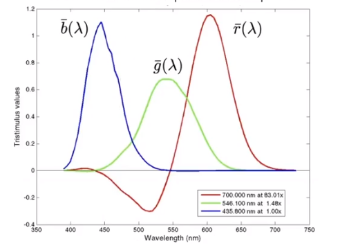
            For any spectrum $s$, the perceived color is matched by the following formulas for scaling the CIE RGB primaries
            $$
            R_{CIE\ RGB}=\int_{\lambda} s(\lambda)\overline r(\lambda)d\lambda
            \\
            G_{CIE\ RGB}=\int_{\lambda} s(\lambda)\overline g(\lambda)d\lambda
            \\
            G_{CIE\ RGB}=\int_{\lambda} s(\lambda)\overline b(\lambda)d\lambda
            $$

      3. Standard Color Spaces

         0. Standardized RGB

            It makes a particular monitor RGB standard, an other color devices simulate that monitor by calibration, a widely adopted today and the gamut（色域） is limited

         1. CIE XYZ

            Imaginary set of standard color primaries X, Y, Z

            0. Primary colors with these matching functions do not exist
            1. Y is luminance（brightness regardless of color）

            Designed such that

            0. Matching function are strictly positive
            1. Span all observable colors

            Separating Luminance, Chromaticity

            Luminance Y, Chromaticity: x, y, z, defined as
            $$
            x=\frac X{X+Y+Z}
            Y=\frac Y{X+Y+Z}
            Z=\frac Z{X+Y+Z}
            $$

            0. Since $x+y+z=1$, we only need to record two of the three
            1. Usually choose $x$ and $y$, leading to $(x,y)$ coords at a specific brightness $Y$

            Then we will get the CIE Chromaticity Diagram

            

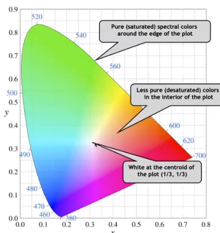
            The curved boundary named spectral locus and it corresponds to monochromatic light（each point representing a pure color of a single wavelength）

         2. Gamut（色域）

            Gamut is the set of chromaticities generated by a set of color primaries. Different color spaces represent different ranges of colors. So they have different gamuts, i.e. they cover different regions on the chromaticity diagram

         3. Perceptually Organized Color Spaces

            0. HSV Color Space（Hue-Saturation-Value）

               Axes correspond to artistic characteristics of color, it is widely used in a “color picker”

               0. Hue（色调）
                  0. the “kind” of color, regardless of attributes
                  1. colorimetric correlate: dominant wavelength
                  2. artist’s correlate: the chosen pigment color
               1. Saturation （饱和度）
                  0. the “colorfulness”
                  1. colorimetric correlate: purity
                  2. artist’s correlate: fraction of paint from the colored tube
               2. Lightness (or value) （亮度）
                  0. the overall amount of light
                  1. colorimetric correlate: luminance
                  2. artist’s correlate: tints are lighter, shades are darker

            1. CIELAB space（AKA L* a * b*）

               A commonly used color space that strives for perceptual uniformiity

               L* is lightness（Brightness）

               a* and b* are color-opponent pairs, a* is red-green and b* is blue-yellow

               Opponent Color Theory

               one piece of evidence: you can have a light green, a dark green, a yellow-green, or a blue-green, but you can’t have a reddish green (just doesn’t make sense). Thus red is the opponents to green

         4. Everything is Relative

         5. CMY A Subtractive Color Space

            Subtractive color model: the more you mix, the darker it will be

            C=Cyan, M=Magenta and Y=Yellow.

            Be careful that there have another name CMYK, but it just used in printing because the color is expensive, black is cheap, but if we use color to get the black, it is dear. So use another K=Key means black can decrease the cost in printing.

10. Animation

“Bring things to life” - Communication tool + Aesthetic issues often dominate technical issues

An extension of modeling - Represent scene models as a function of time

Output: Sequence of images that when viewed sequentially provide a sense of motion

File -24frames per second（FPS）, video（in general）: 30 FPS，virtual reality 90 FPS

History

First Hand-Drawn Feature-Length（>40mins）Animation - Snow White and the Seven Dwarfs

First Digital-Computer-Generated Animation: 1963（vector display）

Early Computer Animation：1972

First CG Feature-Length Film：Toy Story

Keyframe animation

Definition: The most important frame in the sequence of frame which illustrate the most important states.

Keyframe Interpolation: Linear interpolation , splines for smooth / controllable interpolation and etc.

Physical simulation

Newton’s Law $F=ma$

Physically Based Animation: Generate motion of objects using numerical simulation

Mass Spring System

0. A Simple Spring

   Idealized spring（$a,b$ are 2 positions）
   $$
   f_{a\rightarrow b}=k_s(b-a)\\
   f_{a\rightarrow b}=-f_{b\rightarrow a}
   $$
   Force pulls points together, strength proportional to displacement（Hooke’s Low）, $k_s$ is a spring coefficient - stiffness

1. Non-Zero Length spring
   $$
   f(a\rightarrow b)=k_s\frac {b-a}{||b-a||}(|b-a||-l)
   $$
   where $l$ is rest length

2. Introducing Energy Loss

   Simple motion damping $f=-k_d\dot b$

   0. Behaves like viscous drag on motion
   1. Slows down motion in the direction of velocity
   2. $k_d$ is a damping coefficient

   Problem: slow down all motion

3. Internal Damping

   Damp only the internal, spring-driven motion
   $$
   f_b=-k_d\frac {b-a}{||b-a||}(\dot b -\dot a)\frac {b-a}{||b-a||}
   $$
   where $k_d$ is damping force applied on b,$(\dot b -\dot a)$ is the relative velocity of $b$, assuming $a$ is static（vector）, the $\frac {b-a}{||b-a||}(\dot b -\dot a)$ is relative velocity projected to the direction from $a$ to $b$ （scalar）and $\frac {b-a}{||b-a||}$ is direction from $a$ to $b$

   Viscous drag only on change in spring length, it won’t slow group motion for the spring system（e.g. global translation or rotation of the group）

   Note that this is only one specific type of damping

4. Structures from Spring

   Behavior is determined by structure linkages

Particle System

0. Definition

   Model dynamical systems as collections of large numbers of particles.

   Each particle’s motion is defined by a set of physical （or non-physical） forces

1. Popular technique in graphics and games

   0. Easy to understand, implement
   1. Scalable: fewer particles for speed, more for higher complexity

2. Challenges

   0. May need many particles （e.g. fluids）
   1. May need acceleration structures （e.g. to find nearest particles for interactions）

3. For each frame in animation

   0. [If needed] Create new particles
   1. Calculate forces on each particle
   2. Update each particle’s position and velocity
   3. [If needed] Remove dead particles
   4. Render particles

4. Forces

   0. Attraction and repulsion forces
   1. Damping forces
   2. Collisions

Kinematics

0. Forward Kinematics

   0. Articulated skeleton
      0. Topology（what’s connected to what）
      1. Geometric relations from joints
      2. Tree structure （in absence of loops）
   1. Joint types
      0. Pin （1D rotation）
      1. Ball （2D rotation）
      2. Prismatic joint （translation）
   2. Strengths
      0. Direct control is convenient
      1. Implementation is straightforward
   3. Weaknesses
      0. Animation may be inconsistent with physics
      1. Time consuming for artists

1. Inverse Kinematics

   Provide the end point, the procession of arrive to the end point by auto.

   0. Hard
      0. Calculate hard
      1. Multiple solutions
      2. Solutions may not exist
   1. Numerical solution to general N-link IK problem
      0. Choose an initial configuration
      1. Define an error metric （e.g. square of distance between goal and current position）
      2. Compute gradient of error as function of configuration
      3. Apply gradient descent （or Newton’s method, or other optimization procedure）

Rigging

Rigging is a set of higher level controls on a character that allow more rapid & intuitive modification of pose, deformations, expression, etc.

0. Important

   0. Like strings on a puppet
   1. Captures all meaningful character changes
   2. Varies from character to character

1. Expensive to create

   0. Manual effort
   1. Requires both artistic and technical training

2. Blend Shape

   Instead of skeleton, interpolate directly between surfaces.

   Simplest scheme: take linear combination of vertex positions.

   Spline used to control choice of weights over time

Motion Capture

Data-driven approach to creating animation sequences

0. Record real-world performances
1. Extract pose as a function of time from the date collected

Strengths

0. Can capture large amounts of real data quickly
1. Realism can be high

Weaknesses

0. Complex and costly set-ups
1. Captured animation may not meet artistic needs, requiring alterations

Optical Motion Capture

0. Markers on subject
1. Positions by triangulation from multiple cameras
2. Many cameras ,240hz, occlusions are difficult

Challenges of Facial Animation - Uncanny Valley

It is in robotics and graphics. As artificial character appearance approaches human realism, our emotional response goes negative, until it achieves a sufficiently convincing level of realism in expression

Explicit Euler Method

0. single particle simulation

   First study motion of a single particle, later generalize to a multitude of particles.

   To start, assume motion of particle determined by a velocity vector field that is a function of position and time: $v(x,t)$

   

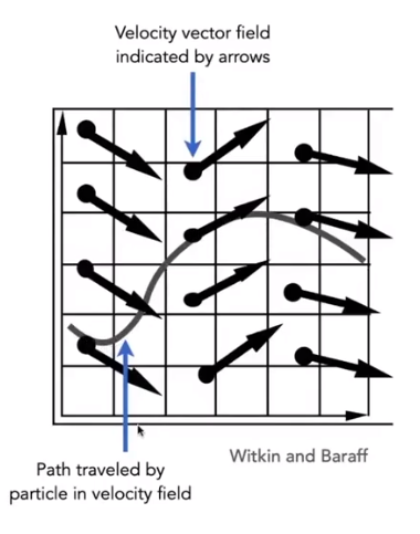
   0. Ordinary Differential Equation（ODE）

      Computing position of particle over time requires solving a first-order ordinary differential equation
      $$
      \frac {dx}{dt}=\dot x=v(x,t)
      $$
      “First-order” refers to the first derivative being taken.

      “Ordinary” means no “partial” derivatives

      Solving for particle position that we can solve the ODE, subject to a given initial particle position $x_0$, by using forward numerical integration.

   1. Euler’s Method

      Euler’s Method （a.k.a. Forward Euler, Explicit Euler）It is a simple iterative method, commonly used, inaccurate and most often goes unstable method
      $$
      x^{t+\Delta t}=x^t+\Delta t\dot x^t\\\dot x^{t+\Delta t}=\dot x^t+ \Delta t \ddot x^t
      $$
      Errors

      With numerical integration, errors accumulate Euler integration is particularly bad,

      

      In stability of the Euler Method

      The Euler method（explicit / forward）: $x^{t+\Delta t}=x^t+\Delta tv(x,t)$

      Two key problems

      0. Inaccuracies increase as time step $\Delta t$ increases
      1. Instability is a common, serious problem that can cause simulation to diverge

      Conclusion of Errors and Instability

      Solving by numerical integration with finite differences leads to two problems

      Errors

      0. Errors at each time step accumulate. Accuracy decreases as simulation proceeds
      1. Accuracy may not be critical in graphics applications

      Instability

      0. Errors can compound, causing the simulation to diverge even when the underlying system dose not.
      1. Lack of stability is a fundamental problem in simulation, and cannot be ignored

   2. Some Methods to Combat Instability

      0. Midpoint method / Modified Euler - Average velocities at start and endpoint

         0. Idea - Compute Euler step, compute derivative at midpoint of Euler step. Then update position using midpoint derivative
            $$
            x_{mid}=x(t)+\frac {\Delta t}2\cdot v(v(x),t)\\
            x(t+\Delta t)=x(t)+\Delta t \cdot v(x_{mid},t)
            $$

         1. Modified Euler - Average velocity at start and end of step. It is better results than before
            $$
            x^{t+\Delta t}=x^t+\Delta t \dot x^t+\frac {(\Delta t)^2}2\ddot x^t
            $$

      1. Adaptive step size - Compare one step and two half-steps, recursively, until error is acceptable

         0. Idea - Technique for choosing step size based on error estimate. It is practical but may need very small steps

            Repeat until error is below threshold

            0. Compute $x_T$ an Euler step, size $T$
            1. Compute $X_{τ/2}$ two Euler steps, size $\frac T2$
            2. Compute error $x_T - x_{T/2}$
            3. If （error > threshold）reduce step size else try again

      2. Implicit methods - Use the velocity at the next time step（hard）

         It is informally called backward methods and use derivatives in the future, fore the current step
         $$
         x^{t+\Delta t}=x^t+\Delta t\dot x^{t+\Delta t}\\\dot x^{t+\Delta t}=\dot x^t+ \Delta t \ddot x^{t+\Delta t}
         $$
         It should solve nonlinear problem for $x^{t+\Delta t}$ and $\dot x^{t+\Delta t}$ but it hard. We can use root-finding algorithm such like Newton’s method, and it will offer much better stability

      3. Position-based / Verlet integration - Constrain positions and velocities of particles after time step

         0. Idea:
            0. After modified Euler forward-step, constrain positions of particles to prevent divergent, unstable behavior. By using constrained positions to calculate velocity
            1. Both of these ideas will dissipate energy, stabilize
         1. Pros / cons
            0. Fast and simple
            1. Not physically based, dissipates energy（error）

      4. Stability
         We use the local truncation error（every step）/ total accumulated error（overall）. It absolute values do not matter, but the orders w.r.t step.

         The implicit Euler has order 1, which means that （h is the step, i.e. $\Delta t$）

         0. Local truncation error: $O(h^2)$
         1. Global truncation error: $O(h)$

         Understanding of $O(h)$ - if we halve $h$, we can expect the error to halve as well

      5. Runge-Kutta Families

         A family of advanced methods for solving ODEs , especially good at dealing with non-linearity. It’s order-four version is the most widely used, a.k.a. RK4
         $$
         y_{n+1}=y_n+\frac 16h(k_1+2k_2+2k_3+k_4)\\
         t_{n+1}=t_n+h
         $$
         where
         $$
         k_1=f(t_n,y_n),k_2=f(t_n+\frac h2,y_n+h\frac {k_1}2)\\
         k_3=f(t_n+\frac h2,y_n+h\frac{k_2}2)\\
         k_4=f(t_n+h,y_n+hk_3)
         $$

Rigid Body Simulation

Simple case: Similar to simulating a particle, just consider a bit more properties

Fluid simulation

0. A Simple Position - Based Method

   Key idea - assuming water is composed of small rigid-body spheres, and the water cannot be compressed.

   So, as long as the density changes somewhere, it should be “corrected” via changing the positions of particles

   You need to know the gradient of the density anywhere w.r.t. each particle’s position and us gradient descent.

1. Eulerian（网格法） vs. Lagrangian（质点法）

   Two different views to simulating large collections of matters.

2. Material Point Method（MPM）

   Hybrid, combining Eulerian and Lagrangian views

   0. Lagrangian: consider particles carrying material properties
   1. Eulerian: use a grid to do numerical integration
   2. Interaction: particles transfer properties to the grid, grid performs update, then interpolate back to particles

OK, 整个课程的知识总结已经完成，现在只剩下一些修补了（主要是一些图还没有上传的图床里面）后续的学习可以考虑 OpenGL或者DirectX，若要学习几何相关，微分几何，拓扑，流形也是需要涉及的；想要对光线更多的了解，可以考虑了解光线与传播。

下一次类似的大型内容应该是基于Python的模拟仿真内容了，六月一号见